TL;DR#
Offline reinforcement learning (RL) aims to learn optimal policies from pre-collected data, without direct interaction with the environment. A major challenge is the sample complexity—how much data is needed—which can scale poorly with the size of the environment. Previous work showed this scaling is unavoidable even with good data coverage (concentrability) and linear function approximation, assuming the data is a sequence of individual transitions.
This paper shows that using trajectory data—sequences of complete interactions—fundamentally changes the problem. The authors prove that under the linear q*-realizability assumption (policy value functions are linear in a feature space) and concentrability, a dataset of size polynomial in the feature dimension, horizon, and a concentrability coefficient is sufficient to learn a near-optimal policy. This result holds regardless of the environment’s size, directly addressing and solving the previously established limitations.
Key Takeaways#
Why does it matter?#
This paper is crucial for offline reinforcement learning (RL) researchers because it overcomes a previously proven impossibility result, demonstrating that statistically efficient offline RL is achievable with trajectory data under realistic assumptions. This opens new avenues for improving offline RL algorithms and advancing the field.
Visual Insights#

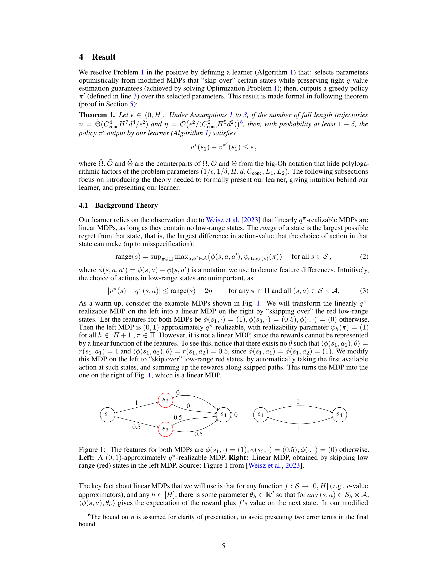
🔼 This figure shows two Markov Decision Processes (MDPs). The MDP on the left is approximately linearly realizable but not linear, while the MDP on the right is linear. The linear MDP is derived from the first by removing (or ‘skipping’) certain states (shown in red). The key idea is that, by carefully skipping over low-range states, a linearly realizable MDP can be transformed into a linear MDP, making the problem of solving it computationally easier. This transformation is central to the algorithm proposed in the paper.
read the caption
Figure 1: The features for both MDPs are $ \phi(s_1,\cdot) = (1), \phi(s_3,\cdot) = (0.5), \phi(\cdot,\cdot) = (0) \text{otherwise. Left: A (0,1)-approximately } q^\pi \text{-realizable MDP. Right: Linear MDP, obtained by skipping low range (red) states in the left MDP. Source: Figure 1 from [Weisz et al., 2023].

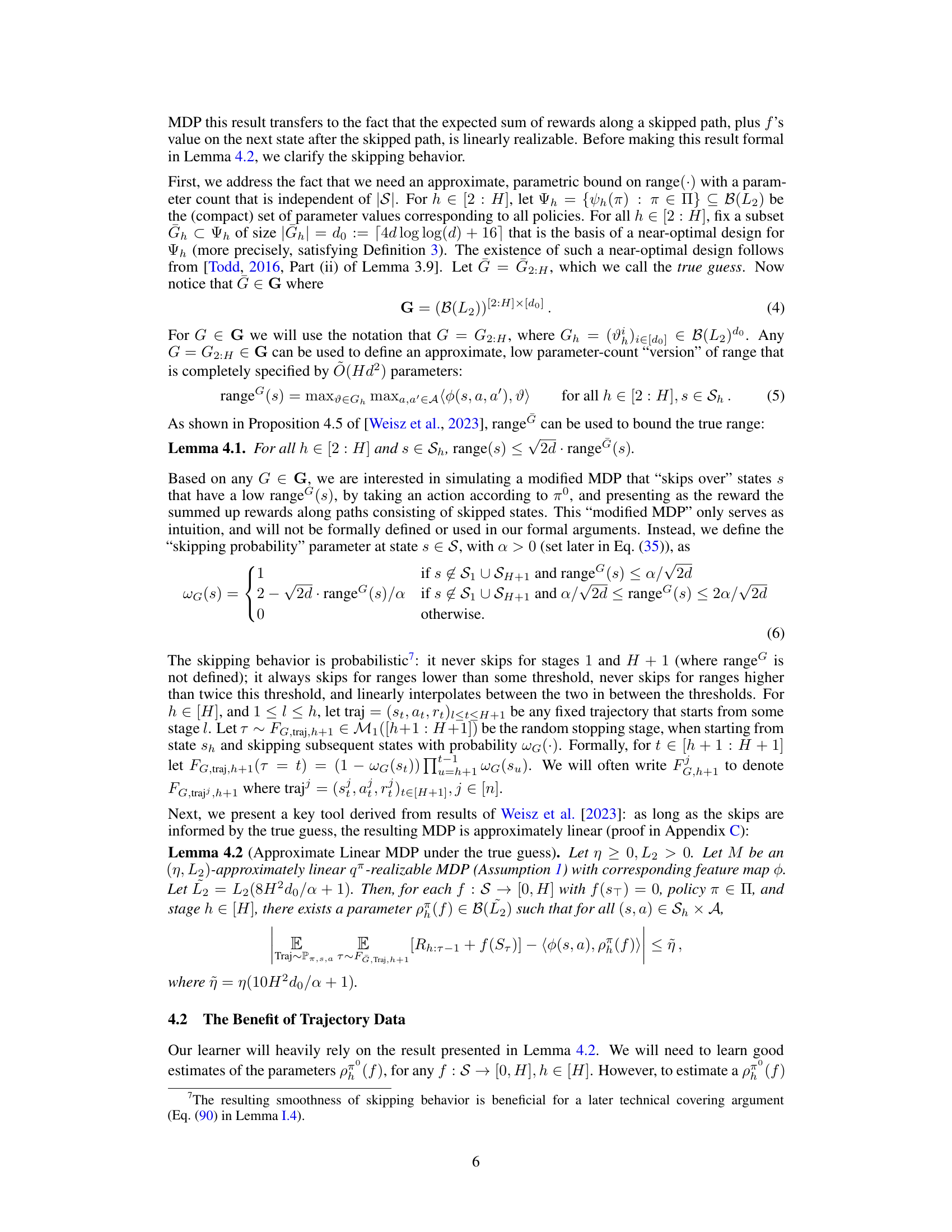
🔼 This table compares the results of the current work with other related works in offline reinforcement learning. It shows the task (policy optimization or evaluation), the type of data used (individual transitions or trajectories), the assumptions made (linear q-realizability, concentrability, and others), and the sample complexity results. A checkmark indicates a polynomial sample complexity, while an ‘x’ indicates an exponential lower bound.
read the caption
Table 1: Notation is defined as: π-opt = policy optimization, π-eval = policy evaluation, Conc = Concentrability, q™ = linear q™-realizability, Traj = Trajectory, √ = poly(d, H, Cconc, 1/€) sample complexity, x = exponential lower bound in terms of one of d, H, Cconc.
Full paper#
