↗ OpenReview ↗ NeurIPS Homepage ↗ Chat
TL;DR#
Estimating the Fisher Information Matrix (FIM) is crucial for understanding and optimizing neural networks, but its high computational cost often necessitates the use of computationally cheaper, diagonal FIM estimators. This study investigates the trade-offs involved in choosing between two popular diagonal FIM estimators, highlighting the variance differences between them.
The paper derives analytical variance bounds for these estimators in neural networks used for both regression and classification tasks. These bounds depend on the non-linearity of the network and the properties of the output distribution. The study concludes that selecting the appropriate estimator involves balancing the trade-off between computational cost and estimation variance, which varies significantly based on factors such as the network architecture, activation function and task type. The paper contributes novel analytical and numerical insights into the practical challenges of FIM estimation in deep learning.
Key Takeaways#
Why does it matter?#
This paper is crucial for researchers working with neural networks. It provides practical tools for efficiently estimating the Fisher Information Matrix (FIM), a key component in understanding and optimizing neural network training. The analytical bounds on FIM variance help researchers select estimators appropriate to their specific scenarios, thereby improving the accuracy and efficiency of optimization. It also opens avenues for research into the effects of FIM estimation variance on optimization algorithms.
Visual Insights#

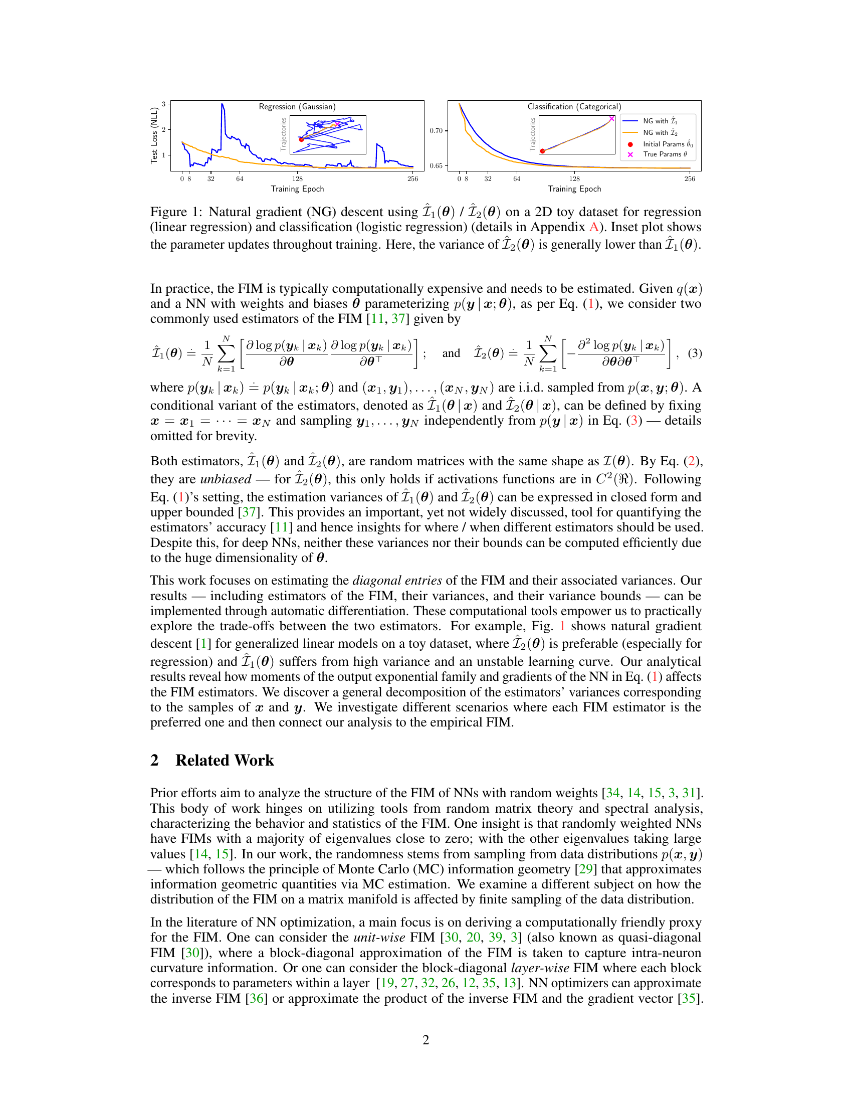
This figure displays the results of a natural gradient descent experiment using two different Fisher Information Matrix (FIM) estimators, Î₁(0) and Î2(0), on a 2D toy dataset. The experiment includes both a regression task (using linear regression) and a classification task (using logistic regression). The main plots show the test loss (negative log-likelihood) over training epochs for both estimators. Inset plots illustrate the parameter updates during training. The caption highlights that the variance of estimator Î2(0) is generally lower than that of Î₁(0).

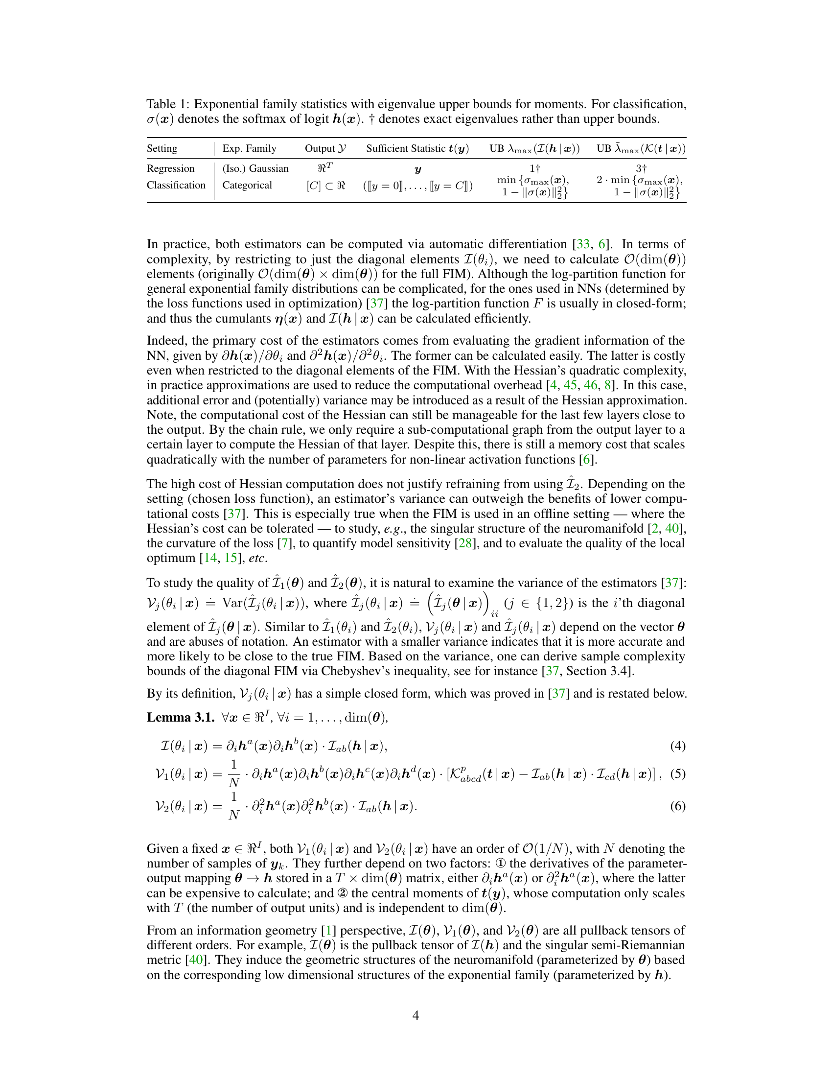
This table presents upper bounds for the maximum eigenvalues of the Fisher information matrix (FIM) and its higher-order moments (specifically the fourth-order moment) for two common exponential family distributions used in machine learning: the Gaussian distribution (for regression) and the categorical distribution (for classification). The upper bounds are given in terms of sufficient statistics of these distributions and highlight the tradeoffs involved in choosing estimators of the FIM based on their respective variances.
In-depth insights#
FIM Estimator Variance#
The Fisher Information Matrix (FIM) is a crucial concept in understanding the geometry of neural network parameter spaces, but its computation is expensive. The paper delves into the variance of FIM estimators, particularly focusing on diagonal entries due to computational constraints. Two popular estimators, Î₁ and Î₂, are analyzed, revealing a trade-off between accuracy and sample complexity. Their variances, derived analytically, depend on the non-linearity of the network and the exponential family distribution of the outputs. Bounds for these variances are provided, offering a practical way to quantify the accuracy of the diagonal FIM estimations. The study highlights that neglecting estimator variance can lead to inaccurate FIM estimates. The variances are shown to depend on the non-linearity with respect to different parameter groups, emphasizing their importance in the estimation process. The findings have implications for optimizing neural network training using techniques like natural gradient descent.
Diagonal FIM Bounds#
The concept of “Diagonal FIM Bounds” in a research paper likely refers to the derivation and analysis of upper and lower bounds for the diagonal elements of the Fisher Information Matrix (FIM). The FIM is a crucial tool in information geometry, characterizing the local geometry of a statistical model’s parameter space. Its diagonal entries represent the individual uncertainties associated with each model parameter. Obtaining bounds is critical because computing the exact FIM is often computationally expensive, especially for complex models like deep neural networks. These bounds provide valuable insights into the accuracy and reliability of estimates of these individual parameter uncertainties. A well-developed analysis would involve mathematical derivations of the bounds, linking them to the model’s structure and the properties of its data distribution. The quality of the bounds would depend on the tightness of the bounds, which would be measured and reported. Ultimately, the presence of tight bounds allows researchers to make more confident conclusions about parameter uncertainty even without the need for computationally expensive direct FIM calculation.
Empirical FIM Tradeoffs#
Analyzing empirical Fisher Information Matrix (FIM) trade-offs involves a nuanced exploration of the balance between computational efficiency and estimation accuracy. Direct FIM calculation is computationally expensive, especially for large neural networks, necessitating the use of estimators which introduce variance. The paper likely investigates the properties of different FIM estimators (e.g., those based on gradients vs. Hessians), evaluating their respective biases, variances, and the influence of various factors such as the neural network architecture (depth, width), activation functions, and the data distribution. A key consideration is how these trade-offs impact optimization algorithms, particularly natural gradient descent methods. The analysis would likely involve theoretical bounds on estimator variance, possibly deriving conditions under which one estimator outperforms another based on the specific problem context. Finally, the paper may present empirical results, demonstrating the observed performance of different estimators on various benchmark tasks, and thus providing practical guidelines for selecting an appropriate FIM estimator given computational constraints and desired accuracy.
Variance in Deep NNs#
Variance in deep neural networks (DNNs) is a critical factor influencing model performance and generalization. High variance can lead to overfitting, where the model performs well on training data but poorly on unseen data. This is because a high-variance model is highly sensitive to the training data’s specific characteristics, effectively memorizing noise instead of underlying patterns. Conversely, low variance can result in underfitting, where the model fails to capture the complexity of the data, resulting in poor performance on both training and test sets. The optimal variance level depends on the dataset’s complexity and the model’s capacity. Regularization techniques, such as dropout and weight decay, aim to reduce variance and improve generalization. Batch normalization helps stabilize the learning process by reducing internal covariate shift and indirectly controlling variance. Understanding and managing variance is crucial for training effective DNNs. Analyzing variance across different layers can also reveal insights into the model’s learning dynamics. Furthermore, variance estimates often serve as crucial components of optimization strategies such as natural gradient descent.
Future Research#
Future research directions stemming from this work on diagonal Fisher Information Matrix (FIM) estimators for neural networks are manifold. Extending the analysis to block-diagonal FIMs would provide more practical estimators for larger networks. The current focus on diagonal elements is a simplification; a full FIM estimate, though computationally expensive, may offer superior results. Investigating the impact of different activation functions and network architectures on estimator variance is crucial for tailoring the approach to specific applications. Connecting the variance of FIM estimators to the generalization performance of neural networks remains an open question, with implications for optimizing training strategies. Furthermore, exploring the relationship between FIM variance and other optimization metrics, such as sharpness or flatness of the loss landscape, could reveal valuable insights into training dynamics and convergence behavior. Finally, developing computationally efficient methods for estimating and bounding higher-order moments of the output distribution would allow for the refinement of the variance bounds and possibly improved estimator design.
More visual insights#
More on figures

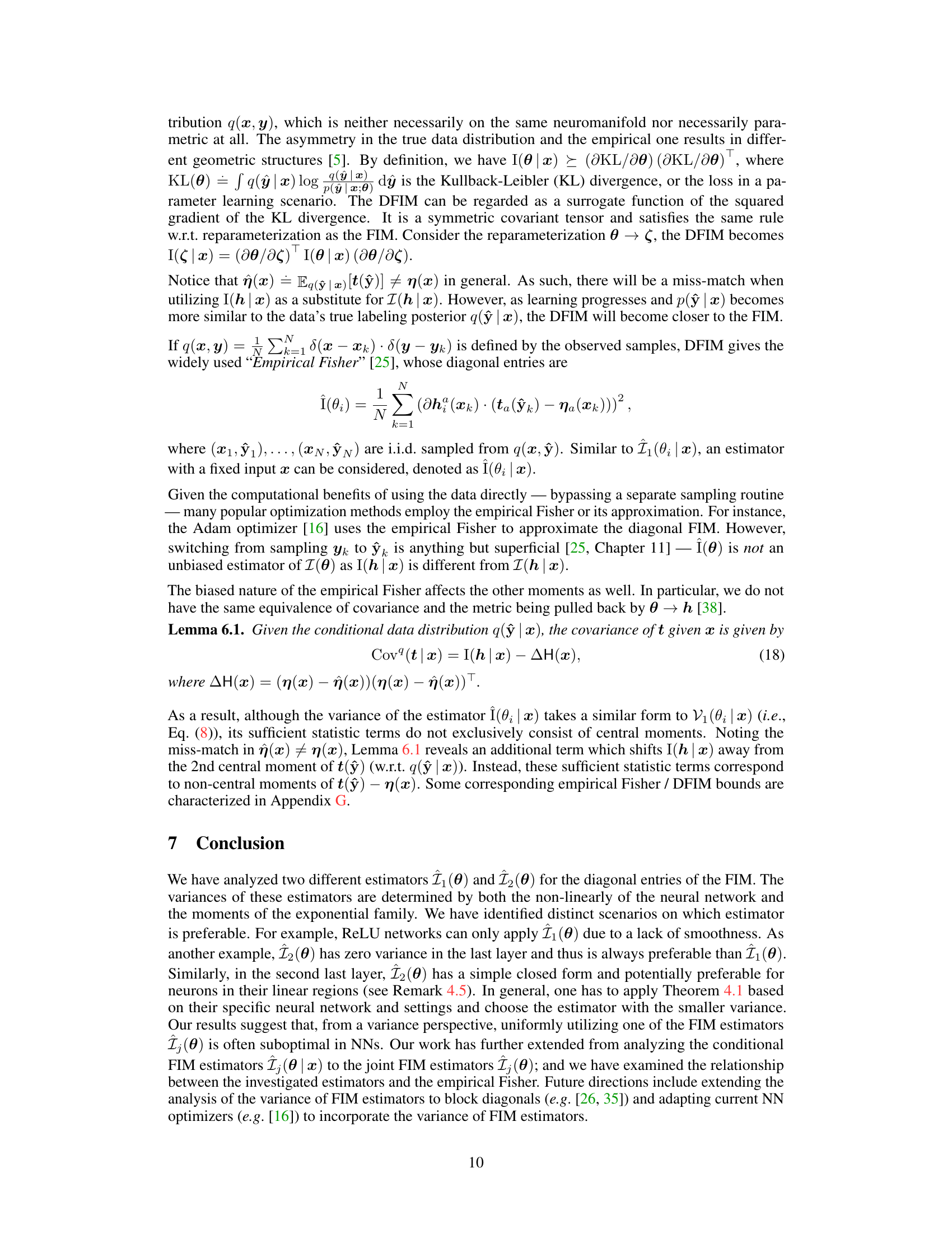
This figure shows the results of an experiment on the MNIST dataset using a 4-layer multi-layer perceptron (MLP) with sigmoid activation functions. The top section plots the estimated Fisher information (FI), along with the standard deviations (square roots of variances) for two different estimators (Î₁ and Î₂) of the diagonal entries of the Fisher Information Matrix (FIM), and their corresponding upper bounds. The bottom section shows the log-ratio between the upper bounds from Theorem 4.1 and the actual variances, indicating the accuracy of these bounds. The results are presented across four parameter groups (one for each layer) over 20 training epochs. The experiment highlights the trade-offs between the two estimators (Î₁ and Î₂) in terms of variance and computational cost, particularly for the last layer where one estimator has a vanishing variance.
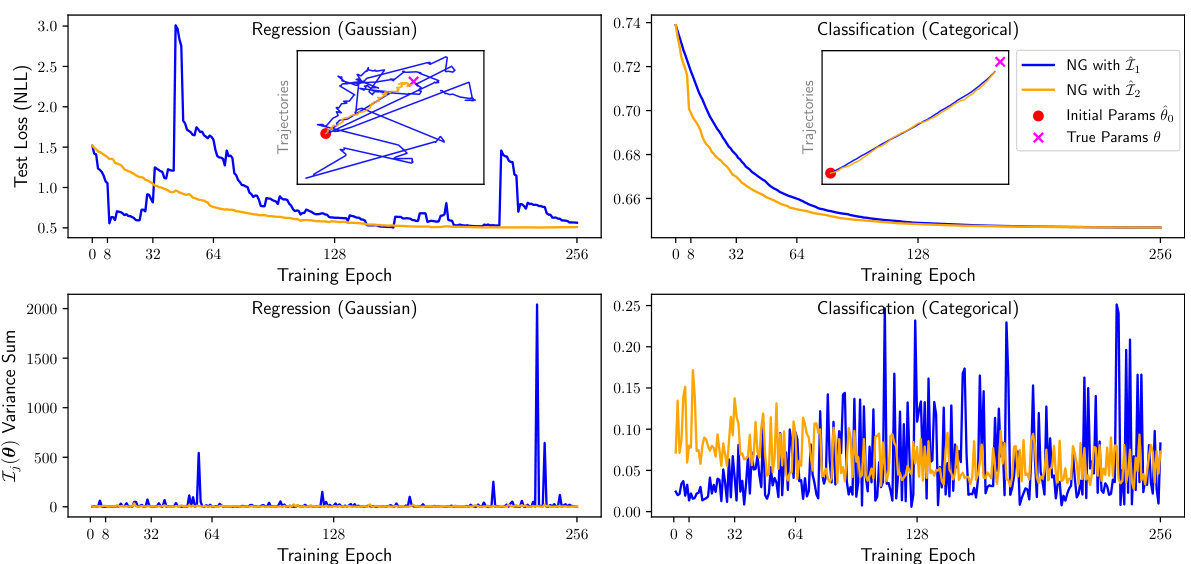
This figure shows the result of applying natural gradient descent using two different FIM estimators (Î₁(θ) and Î₂(θ)) on a simple 2D toy dataset for both regression and classification tasks. The main plots display the test loss over training epochs for each estimator. Inset plots visualize the parameter updates during training. The caption highlights that the variance of Î₂(θ) is generally lower than that of Î₁(θ), suggesting that Î₂(θ) may be a more stable estimator.

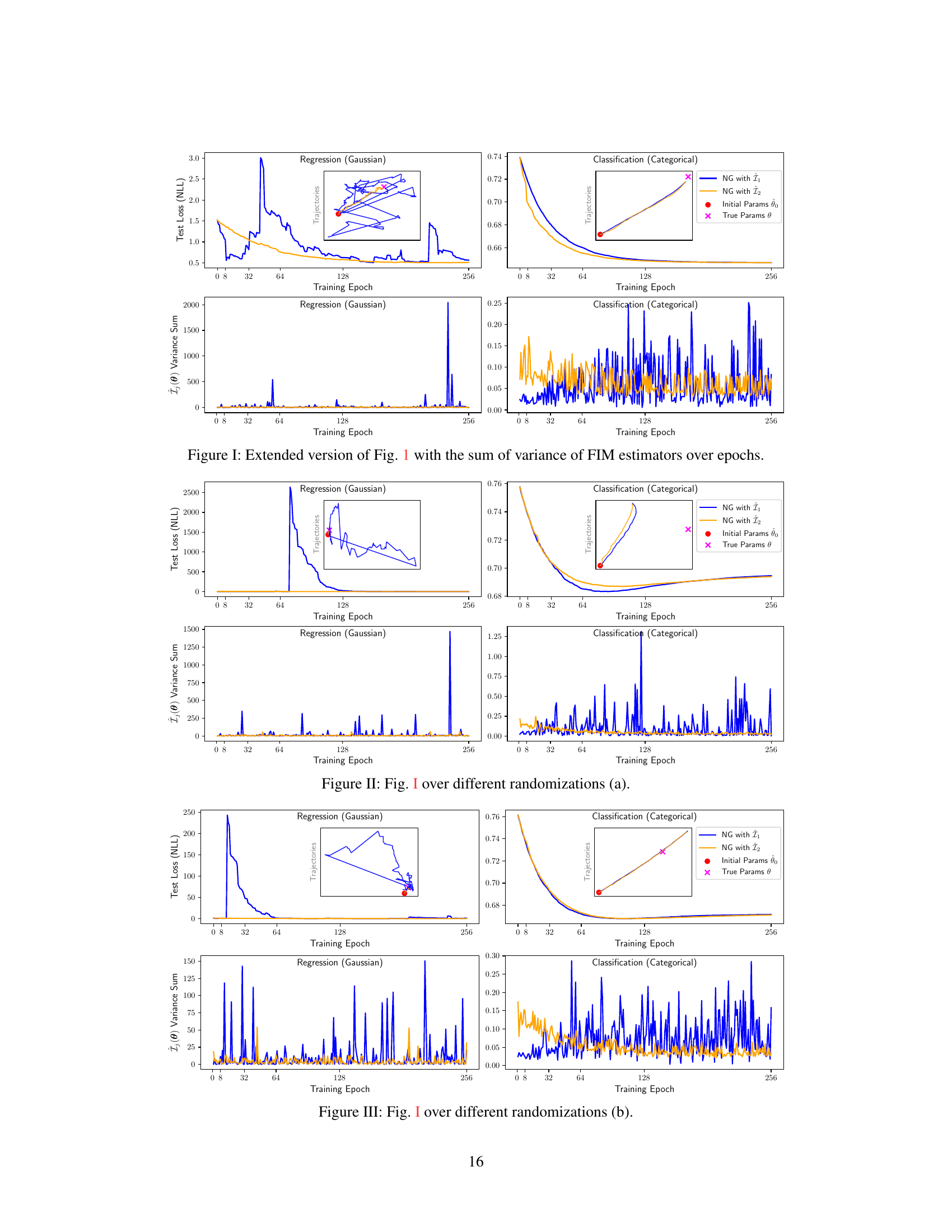
This figure shows the results of natural gradient descent on a 2D toy dataset for both regression and classification tasks using two different estimators of the Fisher Information Matrix (FIM), Î₁(θ) and Î₂(θ). The plot displays the test loss (negative log-likelihood) over training epochs. The inset shows the parameter updates during training, illustrating the trajectories in parameter space. The lower panel shows the sum of variances for the FIM estimators. The results demonstrate that Î₂(θ) generally exhibits lower variance than Î₁(θ), making it a more stable estimator.
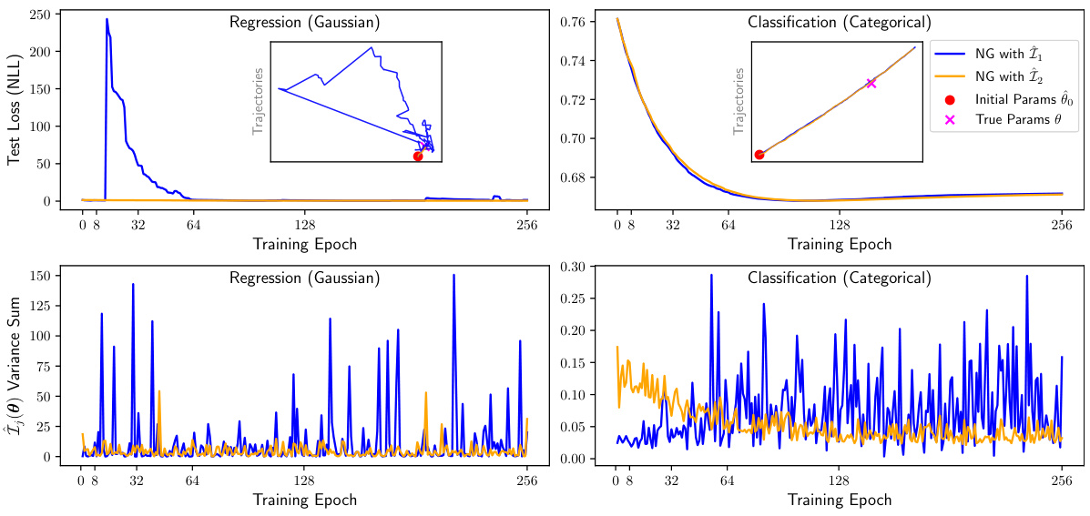
This figure shows the result of natural gradient descent using two different estimators of the Fisher Information Matrix (FIM), Î₁(θ) and Î₂(θ), on a simple 2D toy dataset. The top panels show the test loss for both regression and classification tasks over training epochs. The bottom panels show the variance of the two estimators over the same training period. Inset plots in the top panels visualize the parameter updates during training. The results demonstrate that the variance of Î₂(θ) is generally lower than that of Î₁(θ), suggesting that Î₂(θ) is a more stable and accurate estimator of the FIM in this scenario.
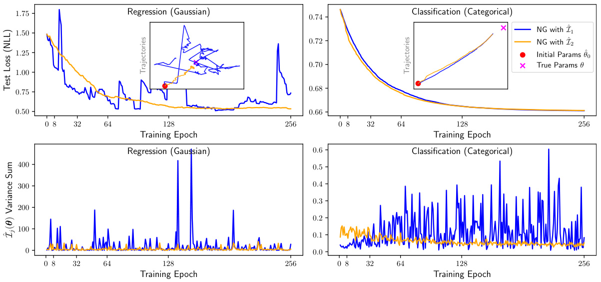
This figure compares the performance of natural gradient descent using two different estimators (Î₁(0) and Î₂(0)) of the Fisher Information Matrix (FIM) for a simple 2D regression and classification task. The left panels show the test loss for both estimators over training epochs. The right panels show the corresponding parameter updates during the training. The inset plots zoom in on the parameter trajectories. The results demonstrate that Î₂(0) generally has lower variance than Î₁(0), making it a more stable estimator.

This figure shows the result of applying two different FIM estimators (Î₁ and Î₂) to the MNIST dataset using a 4-layer MLP with sigmoid activation functions. The top panel displays the estimated Fisher Information (FI), standard deviations of the estimators, and their upper and lower variance bounds across four parameter groups over 20 training epochs. The bottom panel shows the log-ratio of the upper bounds to the actual variances, indicating the tightness of the bounds. Notably, the variance of the second estimator (Î₂) is zero in the last layer, highlighting its superiority in this specific case.

This figure shows the result of an experiment on the MNIST dataset using a 4-layer Multilayer Perceptron (MLP) with sigmoid activation functions. The top part displays the estimated Fisher Information (FI), the standard deviations (square roots of variances) for both estimators (Î₁ and Î₂), and their respective upper bounds. The bottom part shows how close the upper bounds are to the actual variances by plotting the logarithm of their ratio. A ratio close to zero indicates a tight bound. The results are shown for four groups of parameters (one for each layer) over 20 training epochs.

This figure displays the results of an experiment on the MNIST dataset using a 4-layer Multilayer Perceptron (MLP) with sigmoid activation functions. The top section shows the estimated Fisher Information (FI), the standard deviations (square roots of variances) for both estimators (Î₁ and Î₂), and their corresponding upper and lower bounds calculated using Theorem 4.1. The bottom section shows the log-ratio of the upper bounds from Theorem 4.1 to the actual variances, which is a measure of how well the bounds approximate the true variances. The results are presented across four parameter groups (corresponding to the four layers of the MLP) and for 20 training epochs. Note that estimator Î₂ shows zero variance in the last layer, and is not shown in that section.

This figure shows the result of an experiment using the MNIST dataset and a 4-layer Multilayer Perceptron (MLP) with sigmoid activation functions. The top part displays the estimated Fisher Information (FI), the standard deviations (square roots of variances) for both estimators (Î₁ and Î₂), and their upper and lower bounds across four parameter groups over 20 training epochs. The bottom part shows the log-ratio of the theoretical upper bounds (from Theorem 4.1) to the empirical variances, indicating how tight the bounds are. The rightmost column illustrates a situation where the variance of estimator Î₂ is zero, simplifying the analysis.

The figure visualizes the performance of two Fisher Information Matrix (FIM) estimators (Î₁ and Î₂) on the MNIST dataset using a 4-layer Multilayer Perceptron (MLP) with sigmoid activation functions. The top part shows the estimated Fisher Information (FI), their standard deviations (std), and upper bounds across four parameter groups over 20 training epochs. The bottom part displays the log-ratio of the upper bounds from Theorem 4.1 to the actual variances, indicating the tightness of the bounds. The rightmost column highlights that the variance of Î₂ is zero for the last layer, thus its curves are omitted.

This figure displays the results of an experiment conducted on the MNIST dataset using a 4-layer multi-layer perceptron (MLP) with sigmoid activation functions. The top portion of the figure shows the estimated Fisher Information (FI), the standard deviations (square roots of variances) for two different estimators (Î₁ and Î₂), and their upper and lower bounds across four parameter groups over 20 training epochs. The bottom portion shows how close the upper bounds from Theorem 4.1 are to the true variances. A value of 0 means perfect agreement between the bound and the true value. The rightmost column is of particular interest, as it shows estimator Î₂ having zero variance in the final layer.

This figure presents the results of an experiment on the MNIST dataset using a 4-layer MLP with sigmoid activation functions. The top part shows the estimated Fisher Information (FI), the standard deviations (square root of variance) of two different estimators (Î₁ and Î₂), and their corresponding upper and lower bounds calculated using Theorem 4.1, all plotted across 20 training epochs and four parameter groups (one for each layer). The bottom part shows the log-ratio of the theoretical upper bounds from Theorem 4.1 to the actual variances, providing a measure of the tightness of the bounds. Notably, for the last parameter group (rightmost column), the variance of the second estimator (Î₂) is zero, highlighting the differences in variance between the two estimators and the effectiveness of the bounds.

This figure shows the results of an experiment on the MNIST dataset using a 4-layer Multilayer Perceptron (MLP) with sigmoid activation functions. The top part displays the estimated Fisher Information (FI), the standard deviations (square roots of variances) for both estimators (Î₁ and Î₂), and their corresponding upper bounds for each of the four parameter groups across 20 training epochs. The bottom part shows the logarithm of the ratio between the upper bound and the actual variance for each estimator, providing a measure of the tightness of the bounds. The results illustrate how the variances of the estimators behave differently across different layers and epochs and how tightly the derived bounds approximate them.

This figure shows the result of an experiment on the MNIST dataset using a 4-layer multi-layer perceptron (MLP) with sigmoid activation functions. The top section plots the estimated Fisher information (FI), standard deviations (square root of variances) of two different estimators (Î₁ and Î₂), and their upper and lower bounds over 20 training epochs. The bottom section shows how tight the upper bounds are to the true variances. The experiment is broken into four parameter groups corresponding to each of the four layers. The plot highlights that the variance of estimator Î₂ is zero in the final layer and generally smaller than that of estimator Î₁.
Full paper#
