↗ OpenReview ↗ NeurIPS Homepage ↗ Chat
TL;DR#
Disentangled representation learning aims to learn representations where different explanatory factors in data are encoded separately. However, this field lacks clear, universally agreed-upon definitions and reliable evaluation metrics, hindering progress. Many existing metrics don’t clearly quantify what they measure or are difficult to use in model training.
This paper bridges the gap by introducing a novel method for constructing quantitative metrics directly from logical definitions of disentanglement properties. This compositional approach replaces logical operations (equality, conjunction, disjunction, etc.) with quantitative counterparts (premetrics, addition, minimum, etc.) and quantifiers with aggregators (e.g., summation, maximum). The resulting metrics have strong theoretical guarantees and many are easily differentiable, enabling their direct use in learning objectives. Experiments on synthetic and real datasets showcase their effectiveness in isolating different aspects of disentangled representations.
Key Takeaways#
Why does it matter?#
This paper is crucial for researchers in disentangled representation learning due to its novel method for converting logical definitions into quantitative metrics. This method provides strong theoretical guarantees, making it more reliable than existing approaches. The easily computable and differentiable metrics are also valuable for optimization and learning objectives, opening avenues for further research in disentanglement.
Visual Insights#
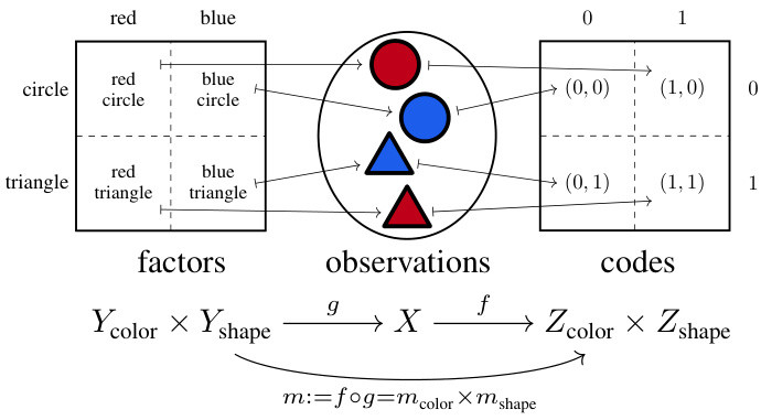
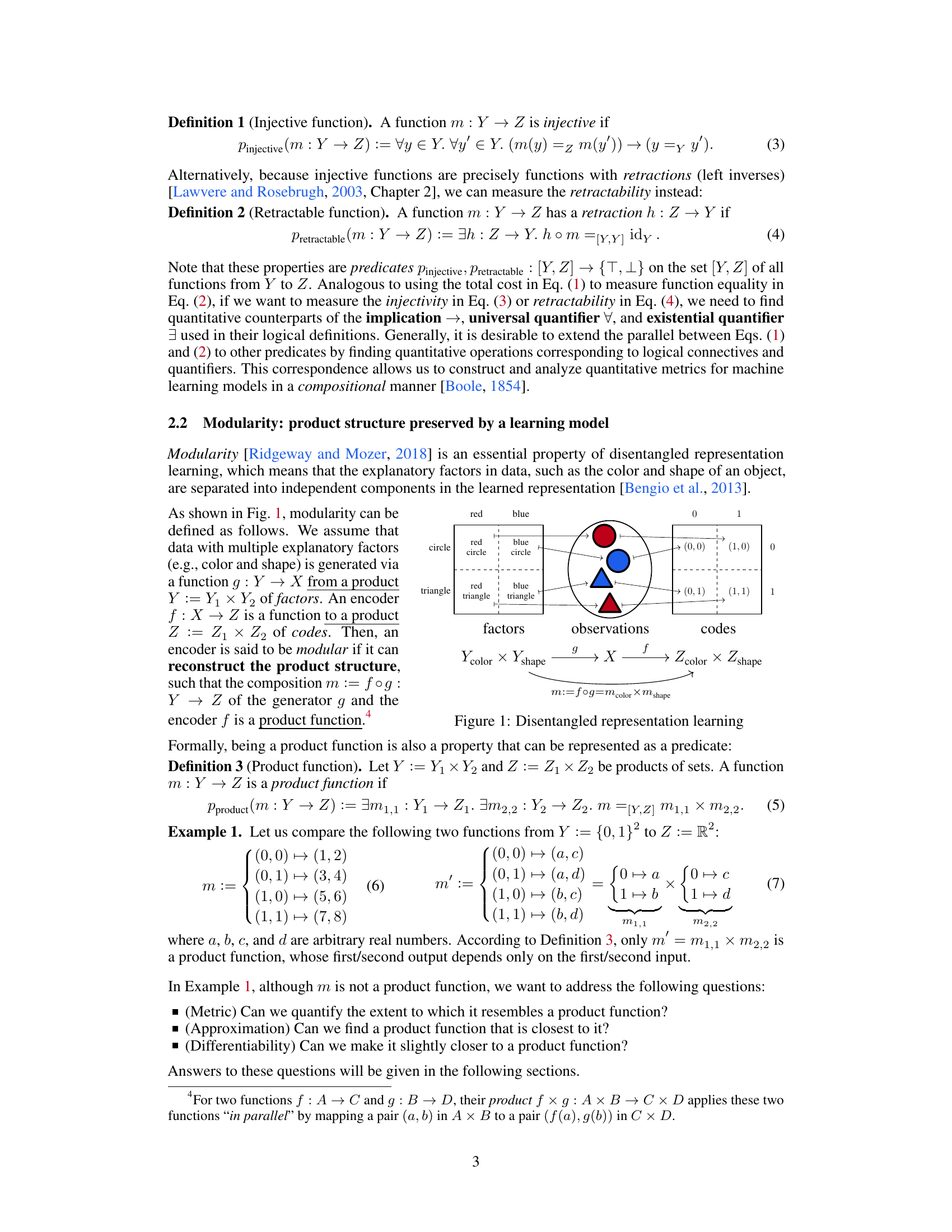
This figure illustrates the concept of disentangled representation learning. It shows data with multiple explanatory factors (e.g., color and shape) being generated via a function g from a product of factor spaces (Y = Y₁ × Y₂). An encoder f maps the observations (X) to a product of code spaces (Z = Z₁ × Z₂). A modular encoder preserves this product structure, meaning that the composition m = f o g of the generator and encoder is a product function. The example shows different combinations of color and shape as inputs, and how a well-disentangled model would represent them as separate factors in the codes.
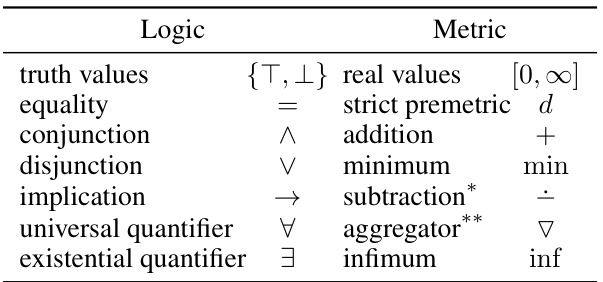
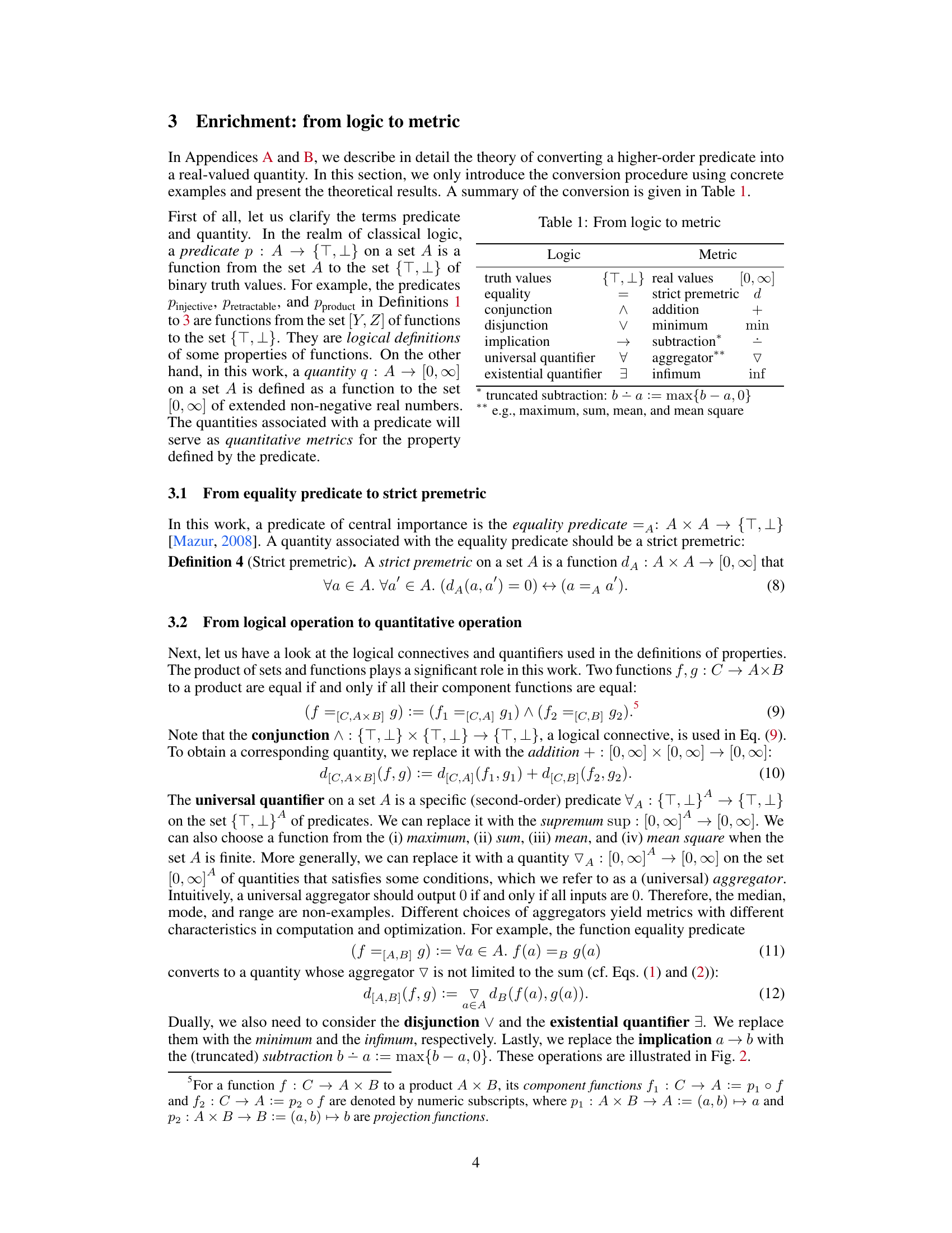
This table summarizes the mapping from logical operations to their corresponding quantitative operations. The left column lists logical concepts (truth values, equality, conjunction, disjunction, implication, universal quantifier, and existential quantifier), and the right column shows their quantitative counterparts (real values [0,∞], strict premetric d, addition, minimum, subtraction*, aggregator**, infimum). The * and ** indicate that the exact operations used may vary based on specific contexts. This mapping is crucial for converting logical definitions of properties into quantitative metrics.
In-depth insights#
Logic-to-Metric#
The core idea of “Logic-to-Metric” is to systematically translate logical properties, often expressed as predicates in formal logic, into quantitative metrics suitable for machine learning applications. This involves a compositional approach where logical connectives (e.g., conjunction, implication) and quantifiers (e.g., universal, existential) are replaced with corresponding quantitative operations (e.g., addition, subtraction, min, max) and aggregators (e.g., summation, supremum). This framework enables a theoretically grounded approach, linking logical definitions of desirable properties (e.g., modularity, informativeness in disentanglement) to real-valued metrics that can be directly used as learning objectives or evaluation measures. A key strength is the provision of theoretical guarantees ensuring that the minimization of a metric implies the satisfaction of the corresponding logical property. However, the use of implication introduces a trade-off, requiring subhomomorphisms to preserve continuity for gradient-based optimization. The practical application demonstrates the effectiveness of this method by creating new disentanglement metrics capable of isolating various aspects of representation learning, surpassing the limitations of previous, less theoretically grounded approaches.
Modularity Metrics#
The research paper explores quantitative metrics for disentanglement in representation learning, focusing on the concept of modularity. Modularity, intuitively, means that different explanatory factors in data are encoded separately. The paper establishes theoretical relationships between logical definitions and quantitative metrics for modularity. Two main approaches are presented for deriving modularity metrics. The first uses a product approximation method, where the goal is to find the product function closest to a given function. This involves optimization but can lead to easily computable and differentiable metrics. The second approach focuses on the constancy of curried functions, eliminating the need for optimization. Different aggregators, such as the mean, variance, or supremum, are used in both approaches, each providing different properties and computational costs. The metrics are evaluated empirically, showing their effectiveness in isolating different aspects of disentangled representations. This section is critical as it bridges abstract logical definitions with concrete, computable metrics that are suitable for both evaluation and training.
Informativeness Metrics#
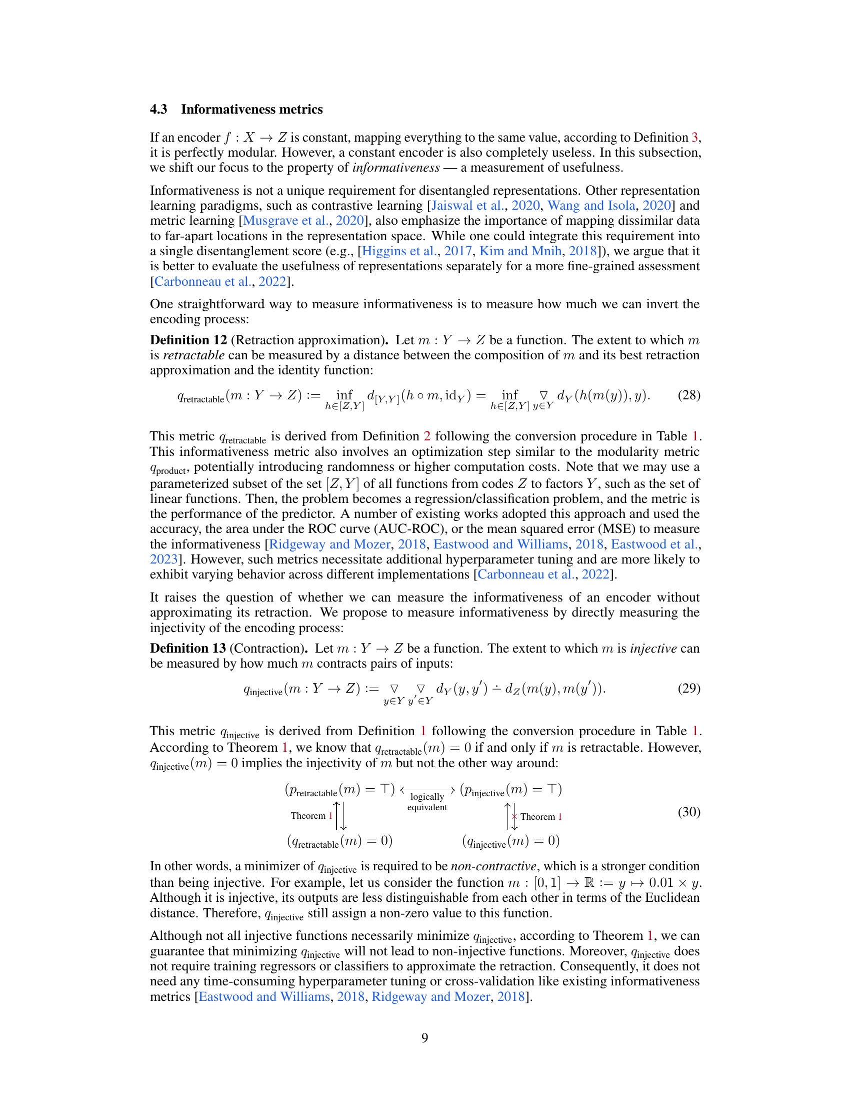
The section on “Informativeness Metrics” explores how to quantitatively assess the usefulness of a representation. Injectivity is highlighted as a crucial aspect, meaning distinct inputs should map to distinct outputs, and a metric is derived to measure this. The concept of retractability is introduced as the ability to reconstruct the original input from its representation. A metric based on how well a representation’s reconstruction approximates the original input is then proposed. The key challenge lies in the computational cost of these metrics. This section also explores the trade-off between theoretically sound but potentially computationally expensive methods and more practical yet less rigorously grounded approximations. The authors emphasize that differentiability is a desirable property for the metrics, enabling their use as direct learning objectives. The focus on easily computable and differentiable metrics reflects a practical approach, balancing theoretical rigor with implementation feasibility.
Experimental Results#
The Experimental Results section of a research paper is crucial for validating the claims made in the introduction. A strong results section will present findings clearly and concisely, using appropriate visualizations like graphs and tables. It’s essential that the results directly address the research questions or hypotheses. Statistical significance should be clearly reported using methods appropriate to the data and analysis. The discussion of results should go beyond simple observation, connecting them to the theoretical framework and prior work. Limitations of the study design should be acknowledged, and potential sources of bias or error discussed. A thoughtful results section enhances the paper’s credibility and impact by providing a thorough and unbiased evaluation of the research findings. Reproducibility is key, so sufficient detail on methodology is needed to allow others to replicate the study. This includes details about data collection, preprocessing, and any specific software or tools used. Finally, a balanced perspective must be maintained, presenting both successful and less successful aspects of the experiments, and analyzing potential reasons for any discrepancies. Only through such comprehensive and rigorous reporting of experimental results can a research paper truly contribute to the field.
Future Directions#
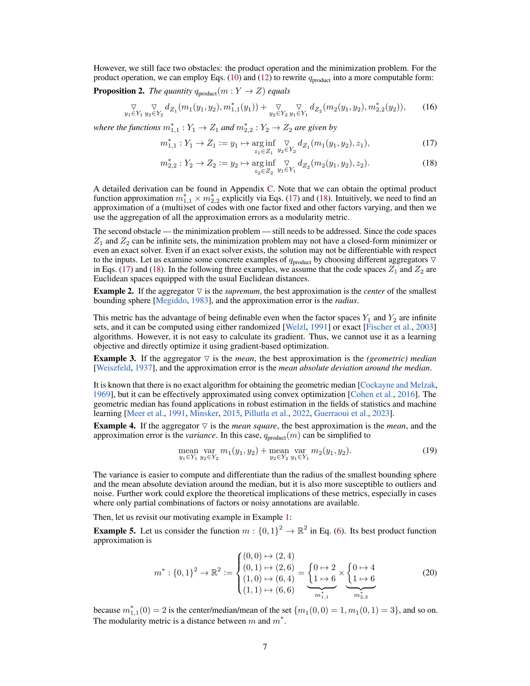
Future research could explore several promising avenues. Extending the framework to handle more complex scenarios such as partial factor observations, noisy data, and multi-modal data is crucial. Developing more sophisticated quantitative metrics that capture nuanced aspects of disentanglement beyond modularity and informativeness is needed. This includes exploring metrics which are computationally efficient and readily differentiable, facilitating direct optimization during the learning process. Investigating the theoretical relationships between the various quantitative measures and exploring ways to combine them into a holistic disentanglement score is also important. Finally, applying this framework to real-world applications and evaluating its effectiveness in practical settings will provide valuable insights into its broader impact.
More visual insights#
More on figures

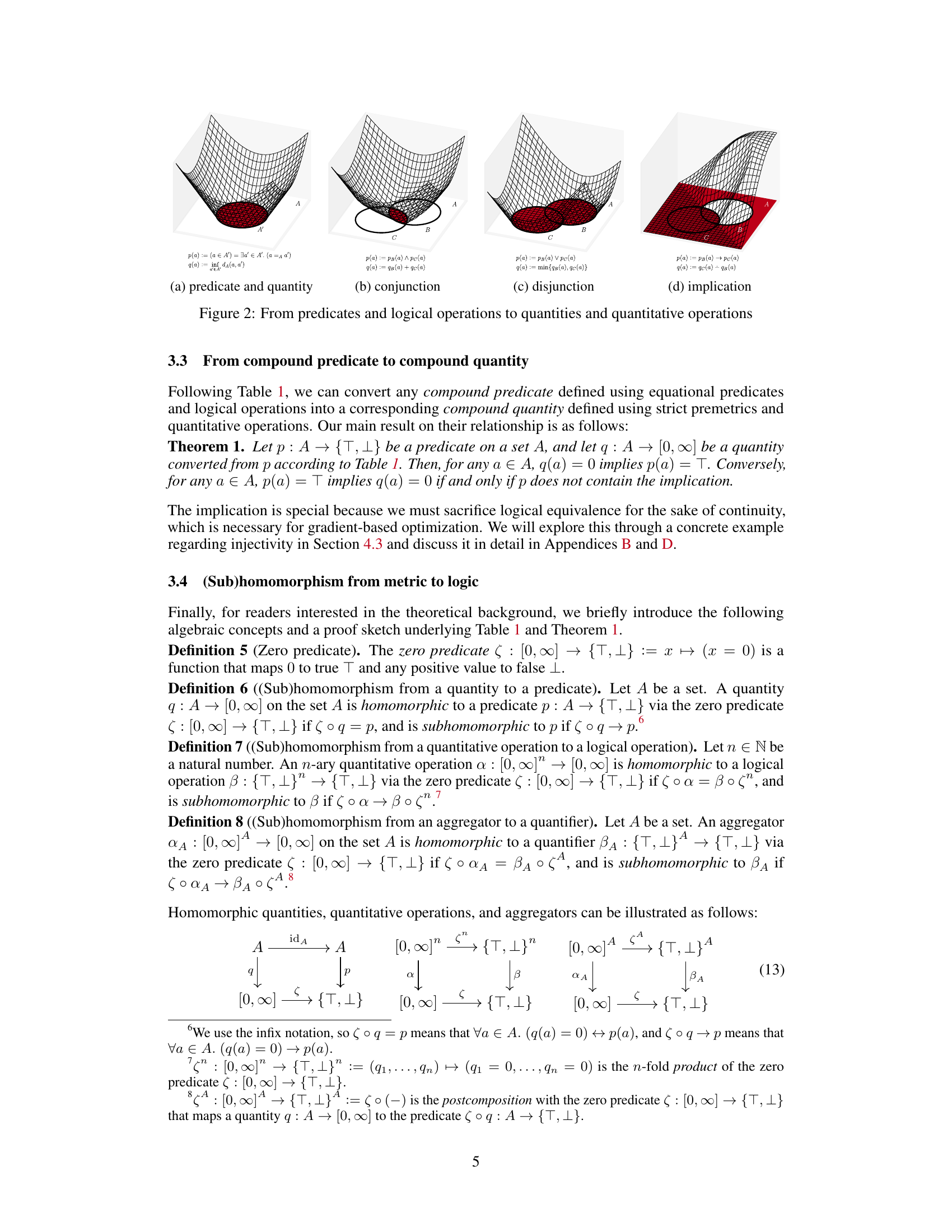
This figure illustrates the compositional approach for converting higher-order predicates into real-valued quantities. It shows how predicates and logical operations (conjunction, disjunction, implication) are converted into quantities and quantitative operations using strict premetrics and quantitative operations. The figure visually represents the relationship between logical definitions and quantitative metrics.

The figure illustrates the concept of disentangled representation learning. It shows data with multiple explanatory factors (e.g., color and shape) being generated by a function g: Y → X, where Y is a product of factor spaces Y = Y₁ × Y₂. An encoder f: X → Z maps the data to a product of code spaces Z = Z₁ × Z₂. The encoder is considered modular if the composition m := f ° g: Y → Z preserves the product structure, meaning m can be decomposed into separate functions m₁,₁: Y₁ → Z₁ and m₂,₂: Y₂ → Z₂.

This figure illustrates the concept of disentangled representation learning using a diagram. It shows how multiple explanatory factors in data (e.g., color and shape) are represented separately in the learned representation. The data is generated via a function g from a product of factors Y. An encoder f maps the observations X to a product of codes Z, where the composition m = f o g is a product function. This demonstrates how disentangled representations preserve the product structure and separate the underlying factors.
This figure illustrates the concept of disentangled representation learning. Data with multiple explanatory factors (e.g., color and shape) is generated by a function g from a product Y of factors. An encoder f is a function that maps the data X into a product Z of codes. A modular encoder is one which preserves the structure of the product (m = f o g).

The figure illustrates the concept of disentangled representation learning. It shows that the data with multiple explanatory factors (e.g., color and shape) are generated via a function g: Y → X from a product Y := Y₁ × Y₂ of factors. An encoder f: X → Z is a function to a product Z := Z₁ × Z₂ of codes. Then, an encoder is said to be modular if it can reconstruct the product structure, such that the composition m := f ◦ g: Y → Z of the generator g and the encoder f is a product function.

The figure illustrates the disentangled representation learning model. The data with multiple explanatory factors (e.g., color and shape) is generated via a function g: Y → X from a product Y:= Y₁ × Y2 of factors. An encoder f: X → Z is a function to a product Z := Z1 × Z2 of codes. Then, an encoder is said to be modular if it can reconstruct the product structure, such that the composition m := f°g: Y → Z of the generator g and the encoder f is a product function.

This figure shows four different functions that could be used as a quantitative operation for negation. The functions are plotted against their input values (n). The red line represents the function [n = 0], which outputs 1 when n is 0 and 0 otherwise. The orange line represents the function 1 ÷ n, which approaches 1 when n is close to 0 and 0 when n approaches ∞. The green line represents the function 1 ÷ n, which shows a similar behavior to the orange line. The blue line represents the function e⁻ⁿ, which decays exponentially as n increases. The choice of which function to use will depend on the specific application and desired properties of the negation operation.
This figure illustrates the compositional approach of converting higher-order predicates into real-valued quantities. It shows how predicates and logical operations (conjunction, disjunction, implication) are converted into quantities and their corresponding quantitative operations by replacing equality with a strict premetric, binary truth values with continuous values, and quantifiers with aggregators. The figure visually demonstrates the transformation process for each logical operation, highlighting the relationship between the logical and quantitative domains.
This figure illustrates the concept of disentangled representation learning. The data, represented by observations (X), is generated by a function (g) that combines multiple explanatory factors (Y1, Y2). An encoder function (f) then transforms the observations into codes (Z), which ideally should maintain the structure of the factors (e.g., as separate components Z1 and Z2). The composition of g and f, denoted as m, which is the path from factors to codes is highlighted, and should also maintain the structure of Y and produce a product function.
The figure illustrates a conceptual model of disentangled representation learning. It shows how multiple explanatory factors (e.g., color and shape) in data are represented separately in a learned representation. The data is initially generated from a product of factors (Y) via a generator (g) resulting in observations (X). An encoder (f) maps these observations to a product of codes (Z). The encoder is considered modular if the composition of the generator and encoder (m) preserves the product structure of the factors. This indicates disentanglement, where different explanatory factors are encoded separately.
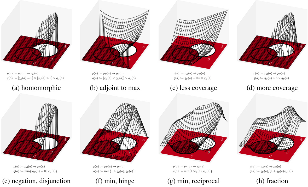
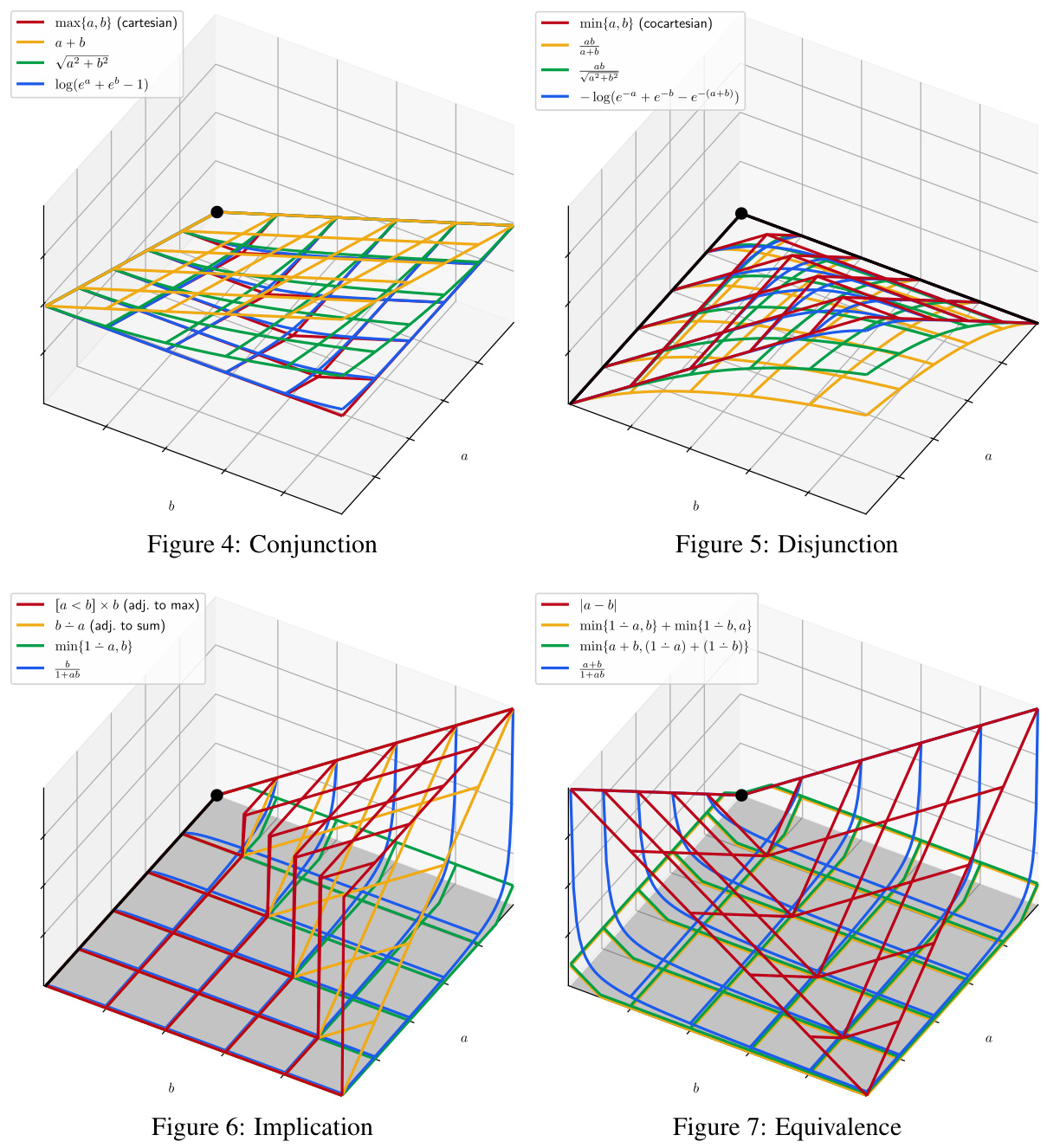
This figure illustrates eight different ways to define a quantitative operation for implication in the context of converting logical definitions into quantitative metrics. Each sub-figure shows a 3D plot representing the quantitative operation’s behavior with respect to the truth values of two predicates (pB(a) and pC(a)) and demonstrates the relationship between these predicates and the quantitative outcomes. The plots show various approaches, from those homomorphic to implication to those using other logical connectives like negation and disjunction, and highlight the differences in their behavior and coverage of possible outcomes.

This figure shows four different quantitative operations for the logical equivalence, which is defined as (a → b) ^ (b → a) (bi-implication), (¬a ∨ b) ∧ (¬b∨ a) (conjunctive normal form (CNF)), (a∧b) ∨ (¬a∧ ¬b) (disjunctive normal form (DNF)). The last one is the fraction operation. Each subfigure shows a 3D plot that visualizes how the value of the quantitative operation changes as the values of the two input quantities vary. The plots showcase the different ways to approximate the logical operation quantitatively.

This figure shows two different approaches to quantify the constancy of a set of points. The first approach involves finding a central point (such as the mean, median, or center of the smallest bounding sphere), and then computing the dispersion around that point. The second approach involves aggregating all pairwise distances between the points in the set. Both approaches aim to quantify how consistent the data points are; high constancy indicates points are clustered tightly, while low constancy suggests a more scattered distribution.

This figure illustrates two different approaches to quantify the constancy of a set of points in a two-dimensional space. The first approach (a) involves identifying a central point (e.g., mean, median, or center of the smallest bounding sphere) and then measuring the dispersion of the points around this central point. The second approach (b) focuses on calculating and aggregating the pairwise distances between all pairs of points in the set.

This figure shows two sets of points. The left one has a small radius and large variance, while the right one has a large radius and small variance. This illustrates how different metrics can rank imperfect representations differently, highlighting the need to consider the characteristics of each metric when choosing one for a specific application.

The figure illustrates that different metrics may rank imperfect representations differently, even if they are derived from the same logical definition. This is because metrics may have different sensitivities to aspects like variance and radius. The top row shows a set of points with a small bounding radius but high variance, while the bottom row shows a set with a larger bounding radius but lower variance. This emphasizes the importance of considering the nuances and characteristics of specific metrics when evaluating disentangled representations.

This figure shows four 3D plots visualizing the transformation of factors to entangled codes and then to approximations. (a) displays the true factors represented using an RGB color cube. (b) shows the entangled codes resulting from an encoder function m: Y → Z, exhibiting a deviation from the perfectly disentangled cube. (c) illustrates a product function approximation attempting to reconstruct a disentangled structure from the entangled codes. Finally, (d) shows a linear approximation of the retraction function h: Z → Y used to reconstruct the factors from the entangled codes.

This figure shows how a standard normal distribution can be transformed into a uniform distribution and vice-versa using probability integral transforms. It further demonstrates how an orthogonal transformation can be used to modify the correlation between variables in the distribution. This illustrates the challenges in disentangling representations, as different transformations can lead to the same or similar distribution.
More on tables

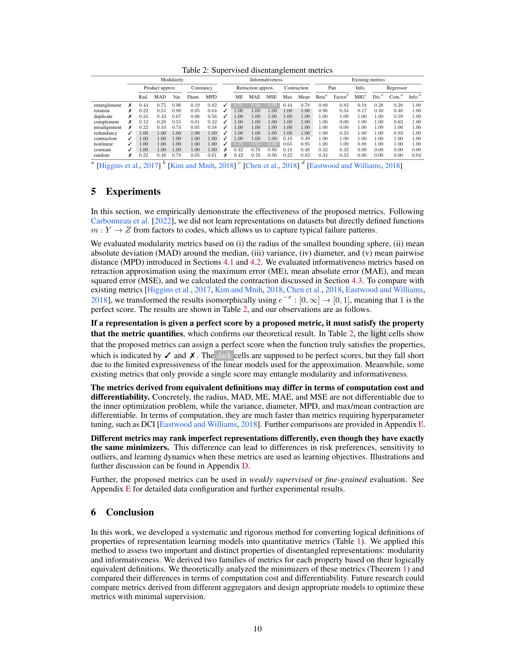
This table presents a comparison of various supervised disentanglement metrics. It shows the performance of different metrics (radius of smallest bounding sphere, mean absolute deviation, variance, diameter, mean pairwise distance, maximum error, mean absolute error, mean squared error, and contraction) on several synthetic datasets representing common failure patterns in disentangled representation learning. The results are scored based on whether the representation satisfies the property the metric is designed to measure, with 1.0 representing perfect results. This allows for a comparison of the effectiveness of the different metrics in isolating different aspects of disentangled representations.

This table presents a comparison of various supervised disentanglement metrics, including those proposed in the paper and existing methods. Metrics are evaluated based on several criteria (radius, mean absolute deviation, variance, diameter, mean pairwise distance, maximum error, mean absolute error, mean squared error, etc.) across different types of representations (e.g., rotation, duplication, misalignment, redundancy). The metrics are categorized into modularity and informativeness, reflecting different aspects of disentangled representation learning.

This table presents the results of evaluating several supervised disentanglement metrics on synthetic data. The metrics evaluated include those based on product approximation (radius, mean absolute deviation, variance, diameter, mean pairwise distance), constancy (radius, mean absolute deviation, variance, diameter, mean pairwise distance), and retraction approximation (maximum error, mean absolute error, mean squared error) as well as a contraction-based metric. The results are shown for various synthetic datasets designed to highlight specific failure patterns in disentangled representations. The datasets include: entanglement, rotation, duplicate, complement, misalignment, and random.
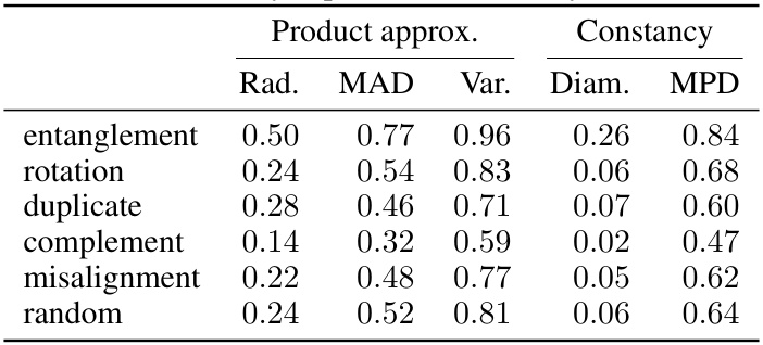
This table presents the results of weakly supervised modularity metrics. It shows the performance of several modularity metrics (radius of the smallest bounding sphere, mean absolute deviation, variance, diameter, mean pairwise distance) on several synthetic data sets representing different types of entanglement of factors.
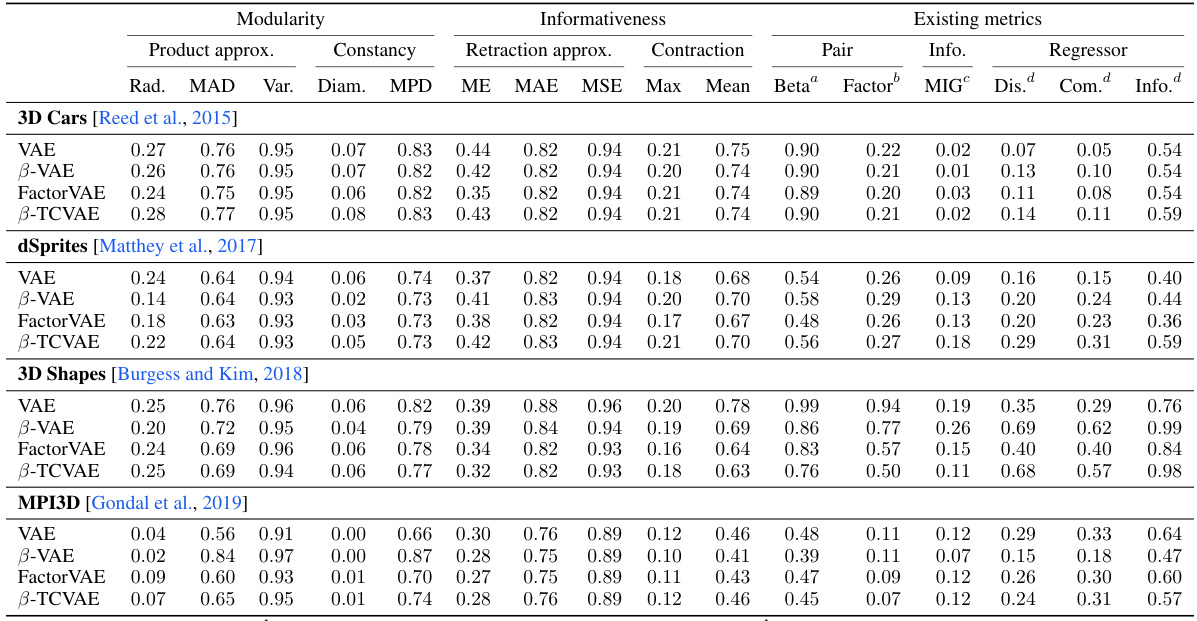
This table presents a comparison of various supervised disentanglement metrics, including both modularity and informativeness metrics. It shows the performance of different metrics on several synthetic datasets designed to capture common failure patterns in disentangled representation learning. The metrics are categorized into product approximation, constancy, retraction approximation, and contraction for modularity and informativeness, respectively. Existing metrics from the literature are also included for comparison.

This table presents a comparison of various supervised disentanglement metrics. It includes metrics based on product approximation, constancy, retraction approximation, and contraction, as well as several existing metrics. The metrics are evaluated across different aspects of disentanglement, such as rotation, duplication, complement, misalignment, and redundancy. The results are presented numerically for each metric and aspect. A checkmark (✓) indicates a perfect score on the metric.

This table presents a comparison of various supervised disentanglement metrics, including both modularity and informativeness metrics. The metrics are evaluated across different datasets (3D Cars, dSprites, 3D Shapes, MPI3D) and failure patterns (entanglement, rotation, duplicate, complement, misalignment, redundancy, contraction, nonlinear, constant, random). The table shows the numerical scores for each metric, facilitating a comparison of their performance and ability to discriminate between different levels of disentanglement.
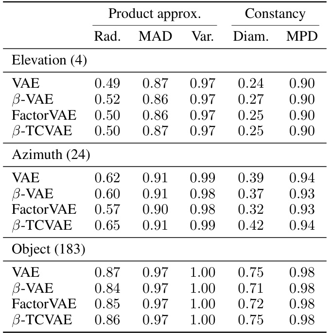
This table presents a comparison of various supervised disentanglement metrics, evaluating both modularity and informativeness aspects. Modularity metrics include product approximation methods (radius, mean absolute deviation, variance, diameter, mean pairwise distance), and constancy metrics. Informativeness metrics include retraction approximation (maximum error, mean absolute error, mean squared error), and contraction. The table also includes several existing metrics for comparison. Results are shown for different simulated scenarios designed to isolate specific aspects of disentanglement.
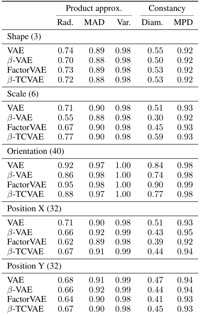
This table presents a comparison of several supervised disentanglement metrics, including both modularity and informativeness metrics. The metrics are evaluated across various synthetic data scenarios designed to isolate different aspects of disentanglement, such as rotation, duplication, and misalignment. Both proposed metrics (derived from logical definitions) and existing metrics from prior work are included for comparison. The results are presented numerically to indicate the degree to which each function satisfies the given property.
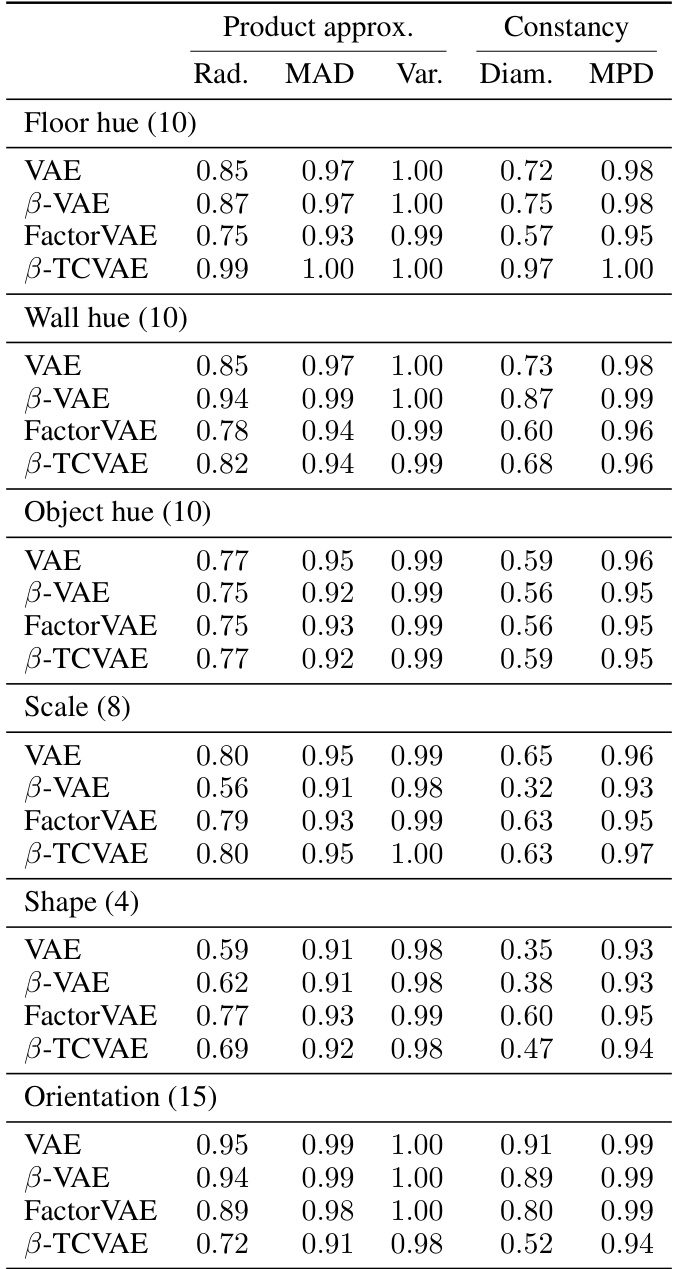
This table presents a comparison of various supervised disentanglement metrics, including both modularity and informativeness measures. The metrics are evaluated across several datasets and compared against existing metrics in the literature. The results show the performance of different metrics in isolating various aspects of disentangled representations.

This table presents a comparison of various supervised disentanglement metrics, including those proposed in the paper and several existing methods. The metrics are evaluated on several synthetic functions designed to highlight various properties and potential weaknesses of disentanglement methods. Different metrics are compared in terms of their ability to isolate and measure different aspects of disentanglement, such as informativeness, modularity, and the tradeoffs between them. The results illustrate how different metrics may rank disentanglement differently and how the proposed metrics are able to achieve a greater level of accuracy in several scenarios.
Full paper#
