↗ OpenReview ↗ NeurIPS Homepage ↗ Chat
TL;DR#
Active learning, while effective, often struggles with real-world complexities such as limited access to data. Existing active learning methods typically assume access to the entire domain, making them impractical for many real-world tasks. This paper addresses this limitation by introducing transductive active learning, where data collection is limited to a sample space while prediction targets reside in a potentially larger target space. This approach is more realistic for settings with constraints and limitations on data acquisition.
This paper presents a novel theoretical framework for transductive active learning, demonstrating its effectiveness through mathematical proofs. It shows that the proposed method, under general regularity assumptions, converges to the smallest attainable uncertainty. Furthermore, the effectiveness of transductive active learning is validated through experiments on active fine-tuning of large neural networks and safe Bayesian optimization, showcasing state-of-the-art performance in both applications.
Key Takeaways#
Why does it matter?#
This paper is crucial for researchers in active learning and related fields because it provides a unified theoretical framework for understanding and improving the efficiency of active learning in complex, real-world scenarios. It bridges the gap between theory and practice by offering theoretical guarantees and demonstrating state-of-the-art performance on multiple real-world applications.
Visual Insights#

This figure shows four different scenarios of transductive active learning, where the goal is to learn a function f within a target space A by actively sampling observations within a sample space S. The four scenarios show how the target and sample space can be related in various ways and how the sampling process can be directed towards specific areas of interest. Scenario A shows a case where the sample space completely covers the target space. Scenario B,C and D demonstrate the scenarios where the sample space does not completely cover the target space and that the sampling process is directed toward learning about a specific target.
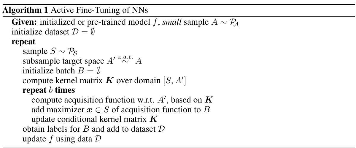
This table summarizes the hyperparameters used in the neural network (NN) experiments described in the paper. It shows the settings for MNIST and CIFAR-100 datasets, including the learning rate, batch size, number of epochs, and other relevant parameters. The asterisk (*) indicates that training continued until convergence on a validation set was achieved.
In-depth insights#
Transductive Learning#
Transductive learning is a powerful machine learning paradigm that bridges the gap between inductive and fully transductive inference. Unlike inductive learning, which aims to generalize from a training set to unseen data, transductive learning focuses on making predictions on a specific, fixed set of test instances. This is particularly useful in scenarios with limited labeled data or high computational constraints, as it reduces the need for extensive model training. A key advantage is its ability to leverage unlabeled data effectively, incorporating information from the entire dataset to improve prediction accuracy on the target examples. However, transductive learning faces challenges in scalability and can be computationally expensive for large datasets. Moreover, theoretical guarantees for transductive learning algorithms are often less established than for inductive methods, posing a challenge to understanding their generalization capabilities. Despite these limitations, transductive learning offers a valuable approach for problems where generalization to unseen examples is not the primary concern. It offers improved sample efficiency and the capability to integrate knowledge from both labeled and unlabeled data, which are significant benefits in many real-world applications.
Active Fine-tuning#
The concept of ‘Active Fine-tuning’ presents a novel approach to enhance the efficiency and effectiveness of model fine-tuning. Instead of passively using all available data, this method actively selects the most informative subset for fine-tuning, thereby significantly reducing computational costs and improving performance. The core idea is to leverage information theory, employing techniques like Information Gain or Variance reduction to guide the selection process. This approach is particularly relevant for large models and/or limited data scenarios, as it optimizes the learning process by focusing on the most beneficial data points. The authors demonstrate the efficacy of this approach in image classification tasks, showcasing superior sample efficiency compared to traditional methods. Furthermore, the integration of pre-trained models and latent structure adds another layer of sophistication, enhancing transferability and generalizability. The theoretical underpinnings of this method are robust, supported by rigorous analysis and convergence guarantees. The potential applications of Active Fine-tuning are widespread and extend beyond image classification, holding promise for various domains where efficient model adaptation is crucial. Active Fine-tuning tackles the challenge of data scarcity and computational expense, offering a pathway towards more effective and resource-conscious machine learning.
Safe Optimization#
Safe optimization tackles the challenge of optimizing objective functions while adhering to safety constraints, a crucial aspect in real-world applications. The core problem involves balancing exploration (searching for better solutions) and exploitation (using currently known safe solutions) while ensuring that no unsafe actions are taken. This is often addressed using methods that build probabilistic models (like Gaussian Processes) of both the objective and the constraints. Active learning plays a key role, as carefully selecting which points to sample next is critical for efficient exploration and effective constraint satisfaction. Transductive active learning extends this by allowing sampling within a restricted safe space (S) to predict the behavior in a larger target space (A), enhancing efficiency when exploring potentially unsafe regions. Algorithms like ITL and VTL are proposed, minimizing posterior uncertainty about the target space, providing theoretical convergence guarantees under specified conditions. Real-world applications such as safe Bayesian optimization and the safe fine-tuning of neural networks demonstrate the effectiveness of these techniques in balancing risk and reward. The key advantage of the transductive approach is its ability to leverage information from safe observations to make informed decisions about potentially unsafe areas, ultimately leading to more sample-efficient and safer optimization processes.
Convergence Rates#
Analyzing convergence rates in machine learning is crucial for understanding the algorithm’s efficiency and reliability. Faster convergence indicates a more efficient learning process, allowing the algorithm to reach a desired level of accuracy with fewer iterations or less data. Slower convergence might point to limitations in the algorithm’s design or the need for more data, potentially impacting the algorithm’s scalability and practical applicability. The theoretical analysis of convergence rates often involves establishing bounds on the error or loss function as a function of the number of iterations, providing insights into the algorithm’s learning dynamics. Tight convergence rates offer a more precise quantification of the algorithm’s efficiency, allowing for a more informed comparison between different algorithms. The choice of metrics used to measure convergence (e.g., error, loss, distance to optimum) impacts the interpretability and significance of the results. Factors influencing convergence rates include the dataset’s characteristics (e.g., size, dimensionality, noise level), the model’s complexity, and the algorithm’s hyperparameters. Empirical evaluation is essential to complement theoretical analysis, validating the theoretical bounds and offering valuable insights into the algorithm’s practical performance in real-world settings. A deeper understanding of these factors and their interplay is critical for improving machine learning algorithms and optimizing their performance.
Future Directions#
Future research directions stemming from this transductive active learning framework are plentiful. Extending the theoretical analysis to broader classes of functions and noise models is crucial for wider applicability. Exploring different uncertainty quantification methods beyond variance and entropy, perhaps leveraging neural network architecture insights, could significantly enhance performance. Investigating adaptive strategies for selecting the target and sample spaces in a data-driven manner would provide greater flexibility and efficiency. Furthermore, it would be beneficial to conduct more in-depth comparisons with alternative active learning strategies tailored for specific domains. Developing efficient algorithms to handle high-dimensional data and large-scale models poses a significant challenge for future work. The proposed framework’s effectiveness across various real-world applications warrants exploring its integration into other machine learning paradigms, such as reinforcement learning and meta-learning, particularly focusing on applications where safety and efficiency are critical constraints, like robotics and healthcare.
More visual insights#
More on figures

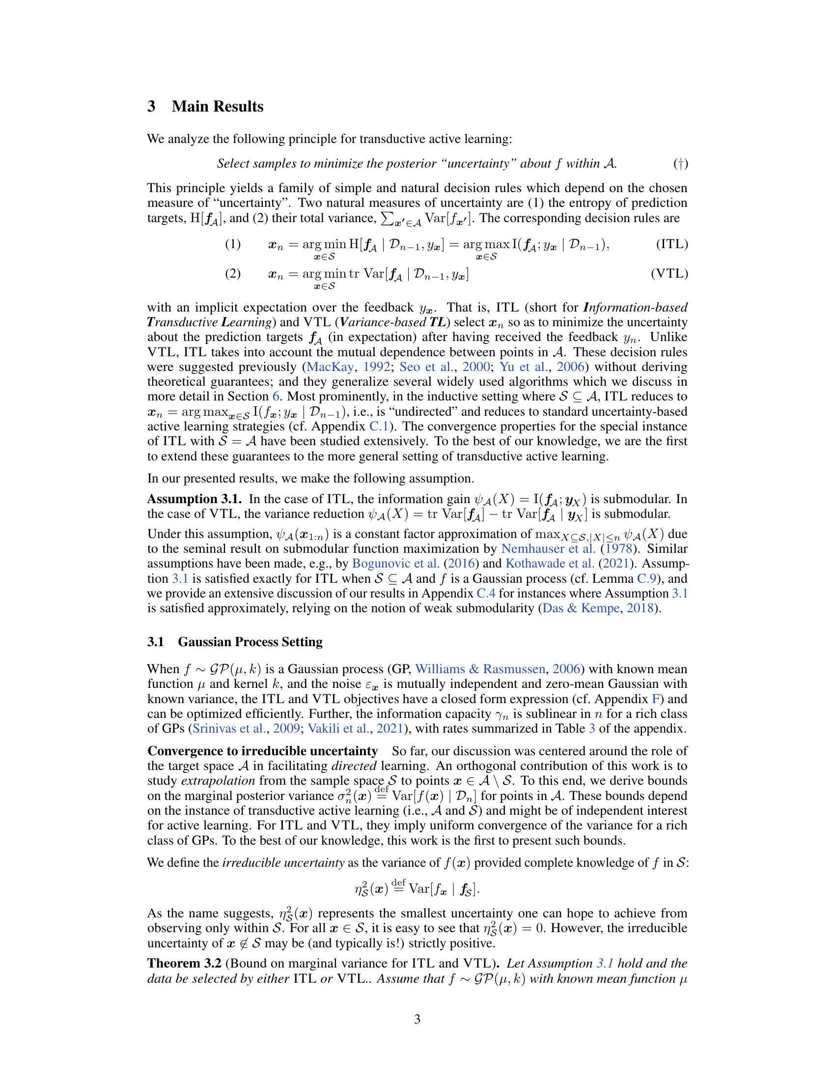
This figure shows examples of how the ITL algorithm selects samples in two different kernel settings (Gaussian and Laplace). The gray area represents the sample space (S), where ITL is allowed to select samples from, and the blue area represents the target space (A), where ITL aims to reduce uncertainty. The plus signs (+) show the 25 initial samples that the algorithm selected. Note that in some cases (three out of the four examples), points outside the target space still contribute useful information for the learning task.

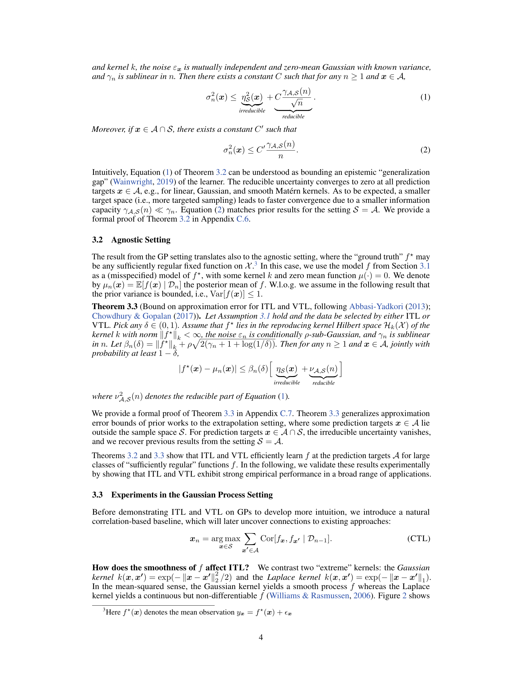
This figure compares the performance of several active learning methods on a Gaussian process regression task. The x-axis represents the number of iterations, while the y-axis shows two different metrics: entropy of fA (left) and mean marginal standard deviation of fA (right). The results demonstrate that Information-Theoretic Transductive Learning (ITL) and Variance-based Transductive Learning (VTL) significantly outperform Uncertainty Sampling (UNSA) and a random baseline. The experiment uses the Gaussian kernel shown in Figure 2(A), where the target space A is a subset of the sample space S.
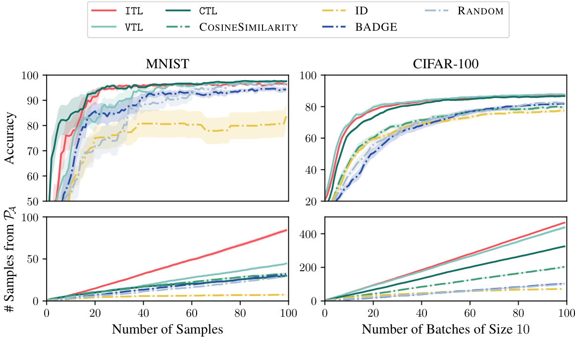
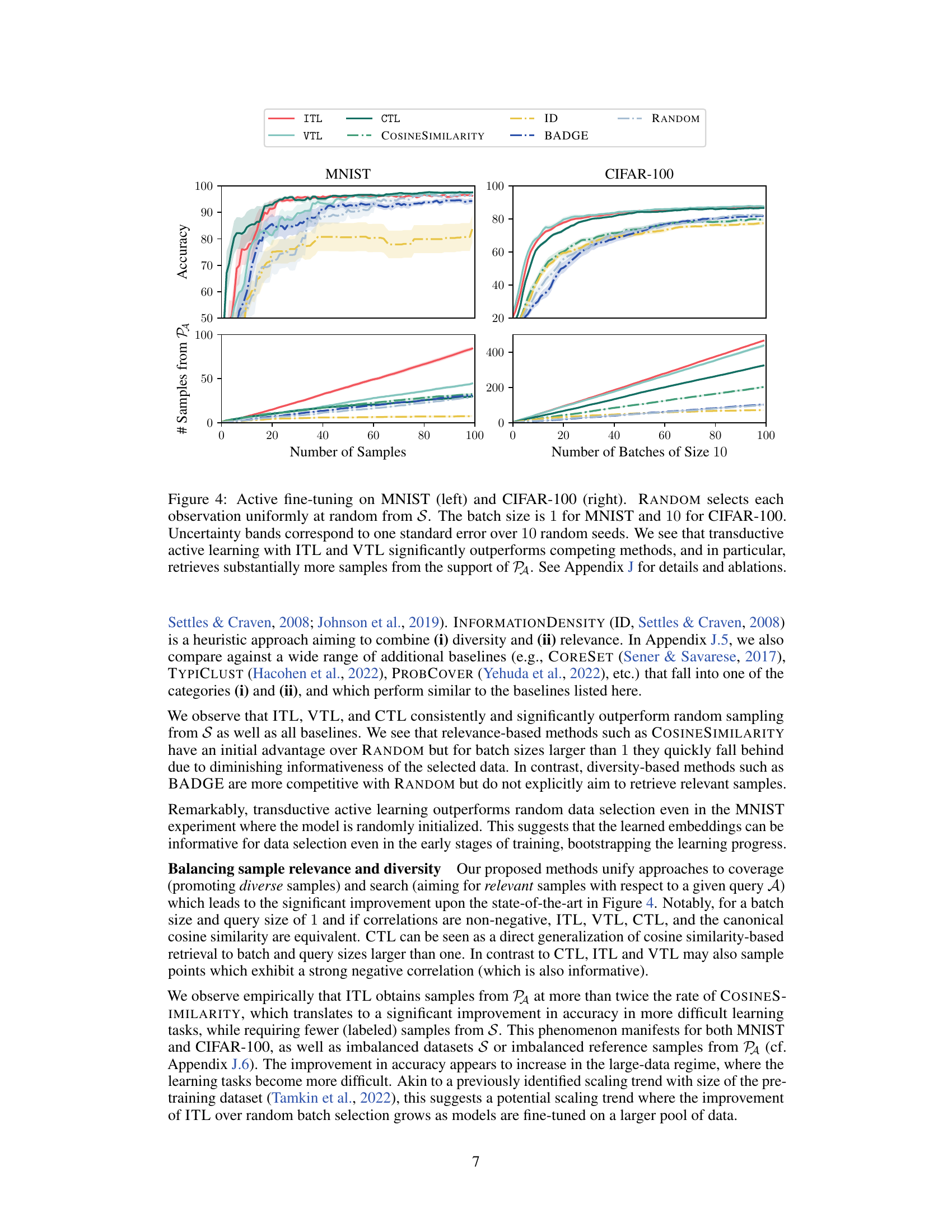
This figure compares the performance of ITL and VTL against several baselines (including random sampling) on MNIST and CIFAR-100 datasets for active fine-tuning of neural networks. The results demonstrate that ITL and VTL significantly outperform the baselines in terms of accuracy and the number of samples retrieved from the support of the target distribution. The y-axis represents accuracy and the number of samples from PA, while the x-axis displays the number of samples and batches respectively. Error bars indicate standard errors across multiple runs.

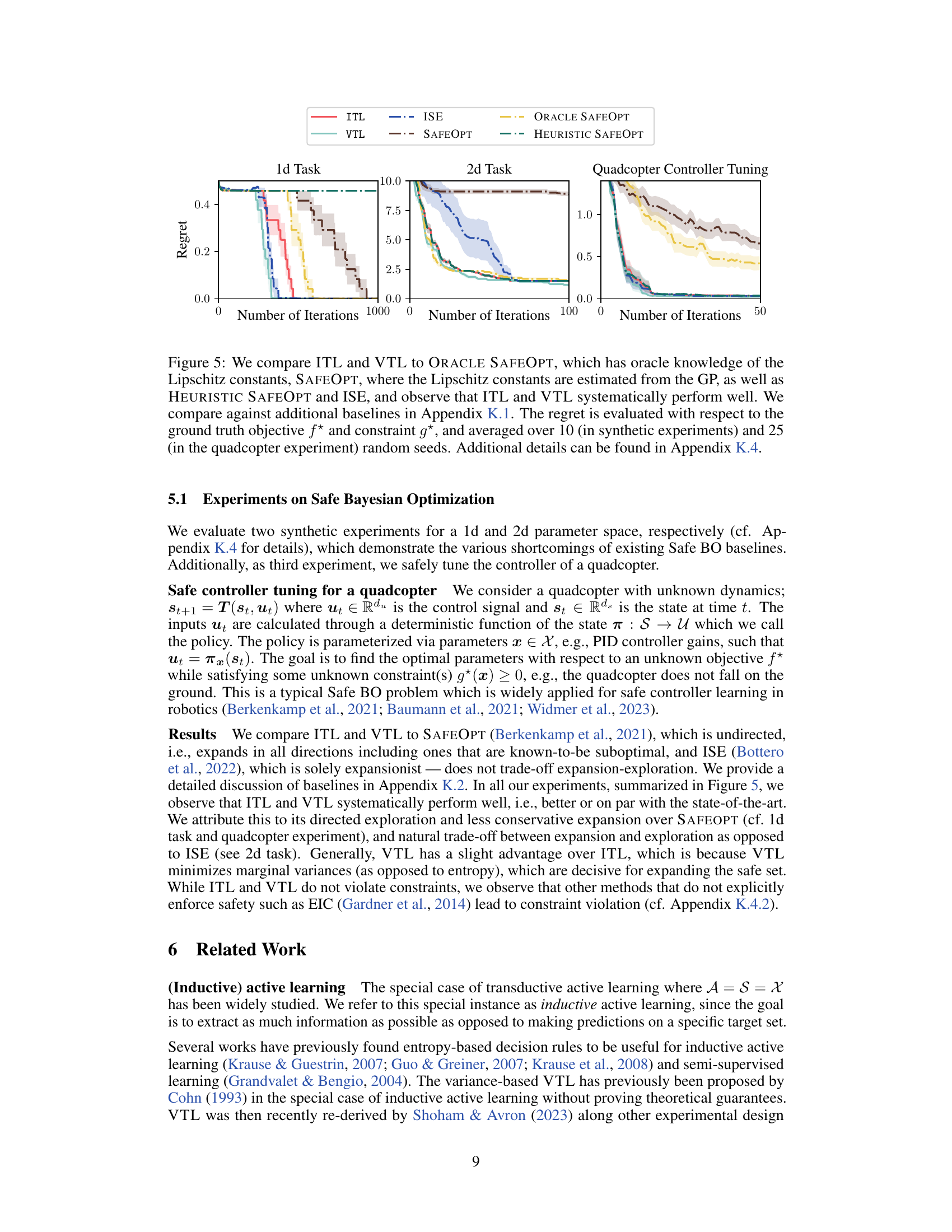
This figure compares the performance of ITL and VTL against several baselines on three different tasks: a 1D synthetic task, a 2D synthetic task, and a quadcopter controller tuning task. The results show that ITL and VTL consistently achieve lower regret, a measure of the difference between the algorithm’s best outcome and the optimal outcome, across all tasks compared to other methods, particularly in scenarios where the Lipschitz constant is unknown or needs to be estimated. This demonstrates the effectiveness of ITL and VTL in finding safe and near-optimal solutions within a limited number of iterations. The use of oracle knowledge, estimated Lipschitz constants, and heuristic methods are also considered and compared.
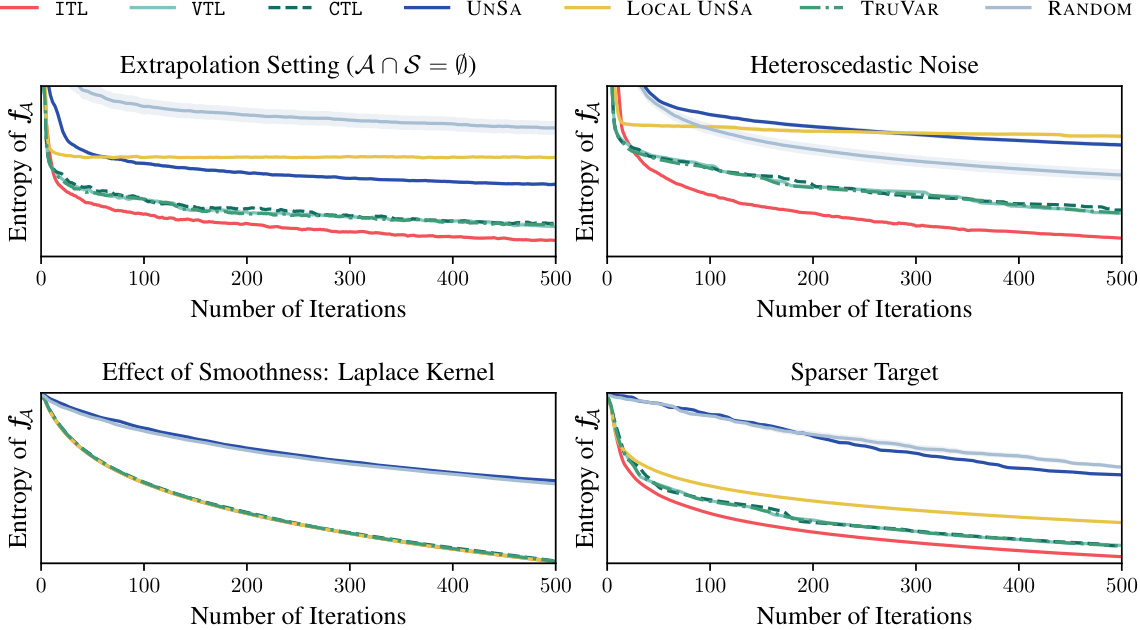
This figure contains four subfigures that show the results of additional Gaussian process experiments. The subfigures illustrate different scenarios: extrapolation (where the target and sample spaces do not intersect), heteroscedastic noise (where the noise variance differs across the domain), the effect of smoothness (using a Laplace kernel), and a sparser target space (with fewer target points). The plots compare the entropy of the target space across several different active learning methods (ITL, VTL, CTL, UNSA, local UNSA, TRUVAR, and random sampling) showing how each method performs under various conditions.

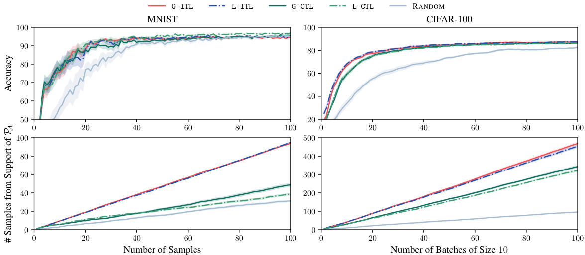
This figure compares the performance of ITL and VTL against other active learning methods and a random baseline for the task of active fine-tuning of neural networks on MNIST and CIFAR-100 datasets. The results show that ITL and VTL significantly outperform other methods, demonstrating their efficiency in selecting informative samples for fine-tuning, and that they select substantially more samples from the relevant part of the data distribution.
This figure compares the performance of ITL and VTL against other active learning methods for the task of active fine-tuning of neural networks on the MNIST and CIFAR-100 datasets. The results demonstrate that ITL and VTL significantly outperform the other methods in terms of accuracy and sample efficiency, especially when considering the proportion of samples selected from the target distribution (PA). The uncertainty bands provide a measure of the variability in the results.

This figure compares the performance of ITL and CTL using two different types of embeddings: loss gradient embeddings and last-layer embeddings. The results are shown for MNIST and CIFAR-100 datasets, and both accuracy and the number of samples from the target distribution are plotted. The goal is to see if using different embeddings changes the performance of the active learning methods.

This figure compares the performance of ITL and VTL against other active learning methods (CTL, UNSA, BADGE, RANDOM, etc.) on the MNIST and CIFAR-100 datasets for the task of active fine-tuning. ITL and VTL consistently outperform the baselines, demonstrating their superior sample efficiency and ability to select relevant samples.
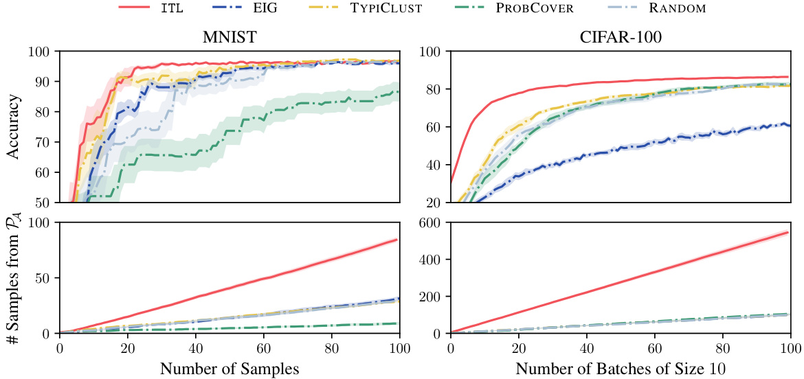
This figure compares the performance of ITL and VTL against several baselines on MNIST and CIFAR-100 datasets for active fine-tuning of neural networks. It shows that ITL and VTL significantly outperform random sampling and other active learning methods in terms of accuracy and the number of samples retrieved from the target distribution PA. Uncertainty bands illustrate the variability of the results. The appendix contains additional experimental details and ablations.
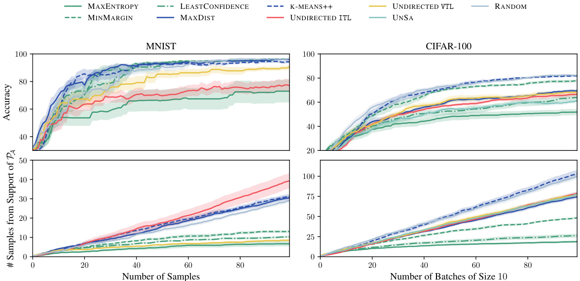
The figure compares the performance of several ‘undirected’ active learning baselines against the ITL and VTL methods on the MNIST and CIFAR-100 datasets. ‘Undirected’ means these methods don’t specifically target a subset of the data (like ITL and VTL do). The plot shows accuracy and the number of samples from the target distribution (PA) obtained over the number of samples or batches. It demonstrates that the directed methods (ITL and VTL) significantly outperform the undirected approaches.
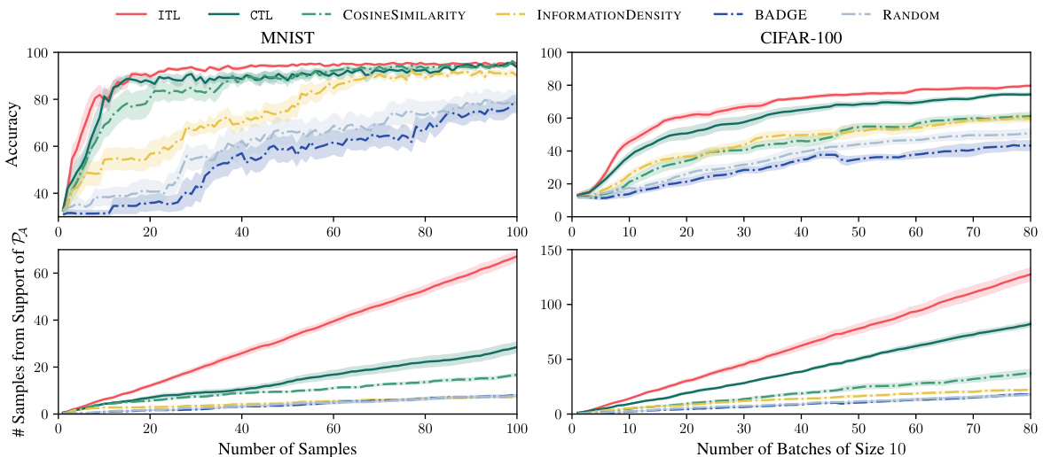
The figure compares different active learning methods on MNIST and CIFAR-100 datasets. ITL and VTL are the proposed transductive active learning methods, while others are baselines. The results show ITL and VTL significantly outperform baselines in terms of accuracy, particularly retrieving more relevant samples. Uncertainty bands represent standard error over 10 runs, illustrating the reliability of results.

This figure compares the performance of ITL and VTL against other active learning methods (CTL, UNSA, BADGE, and RANDOM) on the MNIST and CIFAR-100 datasets. The results demonstrate that ITL and VTL are significantly more sample-efficient in achieving high accuracy, especially when considering the number of samples selected from the target distribution (PA).
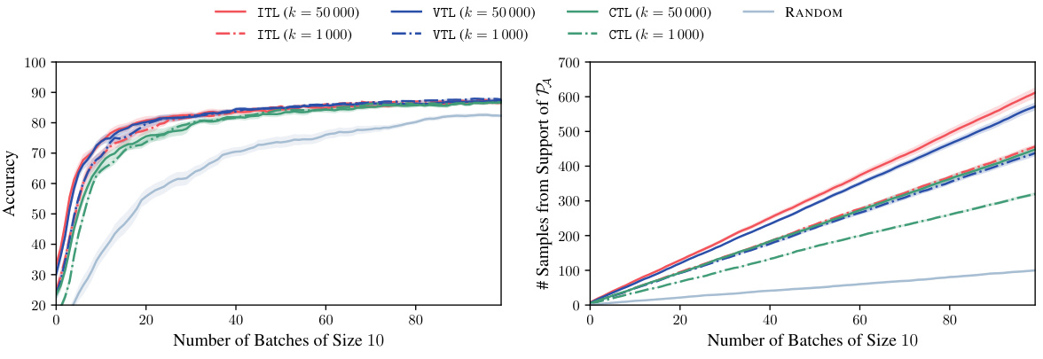
This figure compares the performance of batch selection using conditional embeddings (BACE) against a baseline approach that selects the top-b most informative points according to a decision rule. The results show that BACE significantly improves accuracy and data retrieval, particularly in the CIFAR-100 experiment. This improvement is attributed to BACE’s ability to create diverse and informative batches, unlike the top-b approach which selects points based solely on their individual informativeness without considering the diversity of the batch.

This figure compares the performance of ITL, VTL, CTL, UNSA, BADGE, ID, RANDOM, and COSINESIMILARITY on the MNIST and CIFAR-100 datasets for active fine-tuning. The results demonstrate that ITL and VTL significantly outperform all other methods, achieving higher accuracy with fewer samples from S, particularly retrieving more relevant samples from the support of PA.

The figure shows the performance of ITL with different sizes of the target space A (M = 10, 50, 100, 500) in the CIFAR-100 active fine-tuning experiment. The left panel shows the accuracy on the target dataset, while the right panel shows the number of samples selected from the support of the target distribution. The results demonstrate that larger target space sizes generally lead to better performance, indicating the importance of appropriately sizing the target space for effective active learning.

This figure compares different algorithms for safe Bayesian optimization on three different tasks: a 1D task, a 2D task, and a quadcopter controller tuning task. Each task presents unique challenges in balancing exploration and exploitation while maintaining safety constraints. The algorithms compared are ITL using two different target spaces (An and PAn), VTL using the same two target spaces, and ISE-BO. The use of Thompson sampling introduces stochasticity in selecting target points. The figure showcases the simple regret (a measure of performance in safe BO) over the number of iterations, providing a visual comparison of each algorithm’s convergence and exploration strategy under the different scenarios. Uncertainty bands are also included.
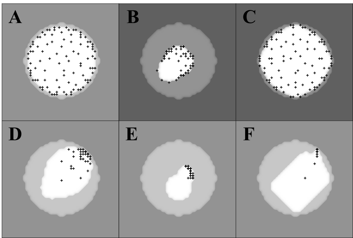
This figure illustrates different scenarios of transductive active learning. The blue area represents the target space (A), where the goal is to learn the function f. The gray area represents the sample space (S), from which observations can be made. Different panels show varying relationships between A and S, including cases where A is fully contained within S, partially overlaps S, or extends beyond S. The key concept is that observations are made within S to improve knowledge about f specifically within A, whereas previous work typically focuses on learning f globally across the entire domain.
This figure shows four different scenarios of transductive active learning, where the goal is to learn a function f in a target space A by sampling from a smaller sample space S. In the first example (A), the target space includes all points in S and also points outside of S. The other examples (B, C, D) show more directed learning, where points are sampled specifically to learn about particular regions or targets within A. The figure highlights that prior work primarily focused on inductive active learning (where A = S), while this paper addresses the more general problem where A and S can be different.

This figure shows a 1D synthetic experiment setup for Safe Bayesian Optimization. The dashed black line represents the true objective function (f*), while the solid black line shows the constraint boundary (g*). The light gray area indicates the initial optimistic safe set (So), meaning regions where the algorithm is initially confident that g*(x) ≥ 0. The darker gray area represents the initial pessimistic safe set, where the algorithm is less certain about the constraint being satisfied. A Gaussian process prior with a linear kernel and sin-transform, along with a mean of 0.1x, is used.

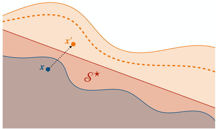
This figure compares the sampling strategies of ITL and SAFEOPT. Both methods aim to solve a safe Bayesian optimization problem. The left panel shows ITL’s sampling, which uses the potential expanders (points that might be safe but aren’t yet known to be) as its target space. In contrast, the right panel illustrates SAFEOPT’s approach, which samples only from the expanders. The figure highlights how ITL can explore more effectively by considering a broader set of potentially safe points, enabling it to overcome local barriers and discover globally optimal solutions more quickly than SAFEOPT, which focuses its exploration only on points already deemed close to being safe.
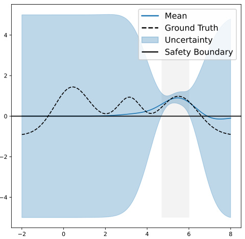
The figure shows the ground truth function (dashed black line), a well-calibrated GP model (blue line with shaded uncertainty region), and a safety constraint (black horizontal line). The light gray area represents the initial safe region S0 where the algorithm can safely explore before learning. The goal is to maximize the objective function while remaining in the safe region.

The figure shows the results of active fine-tuning experiments on MNIST and CIFAR-100 datasets. It compares the performance of ITL and VTL against several baselines, including random sampling. The results demonstrate that transductive active learning using ITL and VTL significantly improves sample efficiency and outperforms other methods in terms of accuracy.

The figure shows the ground truth of the objective and constraint functions in the 2d synthetic experiment. The objective function has two local maxima, while the constraint function defines a circular safe region. The visualization helps understand the complexity of the optimization problem and how the algorithm navigates the safe region to find the optimal solution.
More on tables

This table summarizes the hyperparameters used in the neural network (NN) experiments described in the paper. It lists the values for standard deviation of noise (ρ), the size of the target set (M), the number of samples in the target space (m), the size of the candidate set (k), batch size (b), number of epochs, and the learning rate for both MNIST and CIFAR-100 datasets. The (*) indicates that for MNIST, training continued until convergence on the oracle validation accuracy was reached.
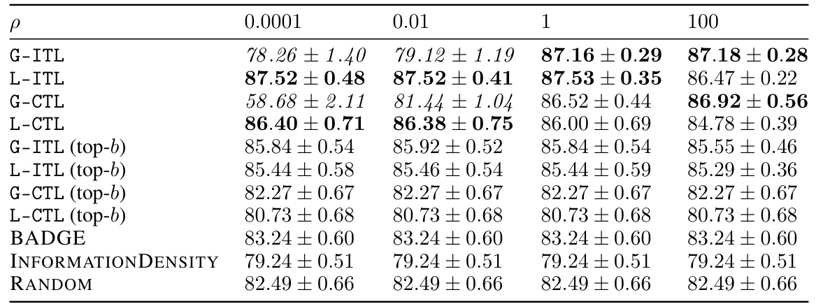
This table presents an ablation study on the effect of noise standard deviation (p) on the performance of different active learning algorithms for the CIFAR-100 dataset. It shows the accuracy achieved after 100 rounds of selection, along with standard errors across 10 random seeds. The table compares the performance of ITL, VTL, CTL and several baselines, both with and without top-b batch selection. Bold values indicate top performance, and italicized values highlight results affected by numerical instability.
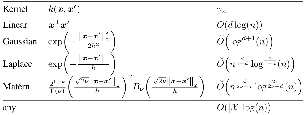
This table shows the upper bounds on the information gain for different kernels, which is useful for analyzing the sample complexity of active learning algorithms. The bounds are given in terms of the number of samples (n) and the dimensionality (d) of the input space. The table also notes the relationship between Matérn and Laplace/Gaussian kernels.
Full paper#


