TL;DR#
Many deep learning applications rely on adaptive stochastic gradient descent (SGD) algorithms, but existing theoretical analyses often assume unbiased gradient estimators—an unrealistic assumption in several modern applications using Monte Carlo methods. This creates a crucial gap in our theoretical understanding of these widely-used algorithms’ behavior. The lack of theoretical guarantees for biased estimators limits the development of more robust and efficient deep learning models and hinders a more complete understanding of their behavior in real-world applications.
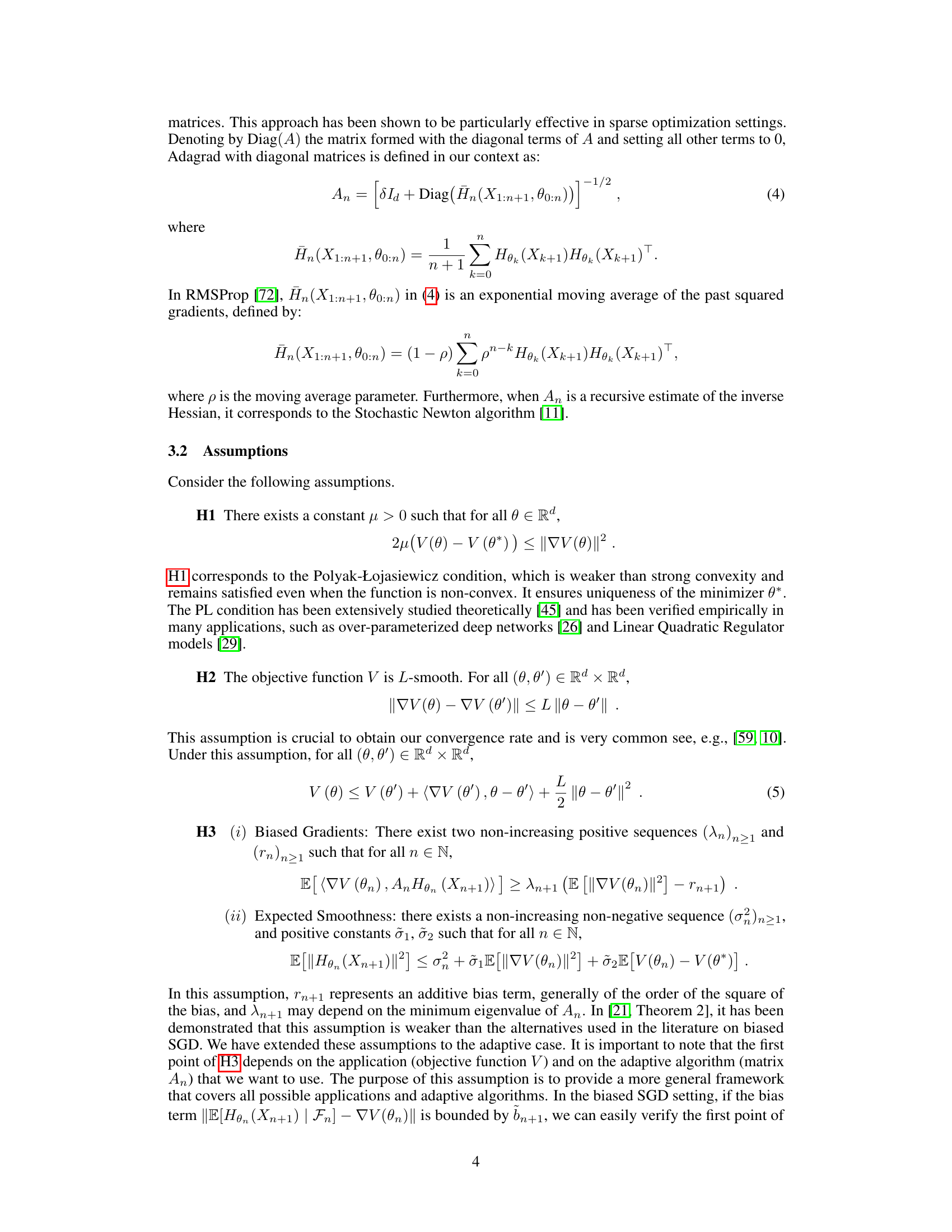
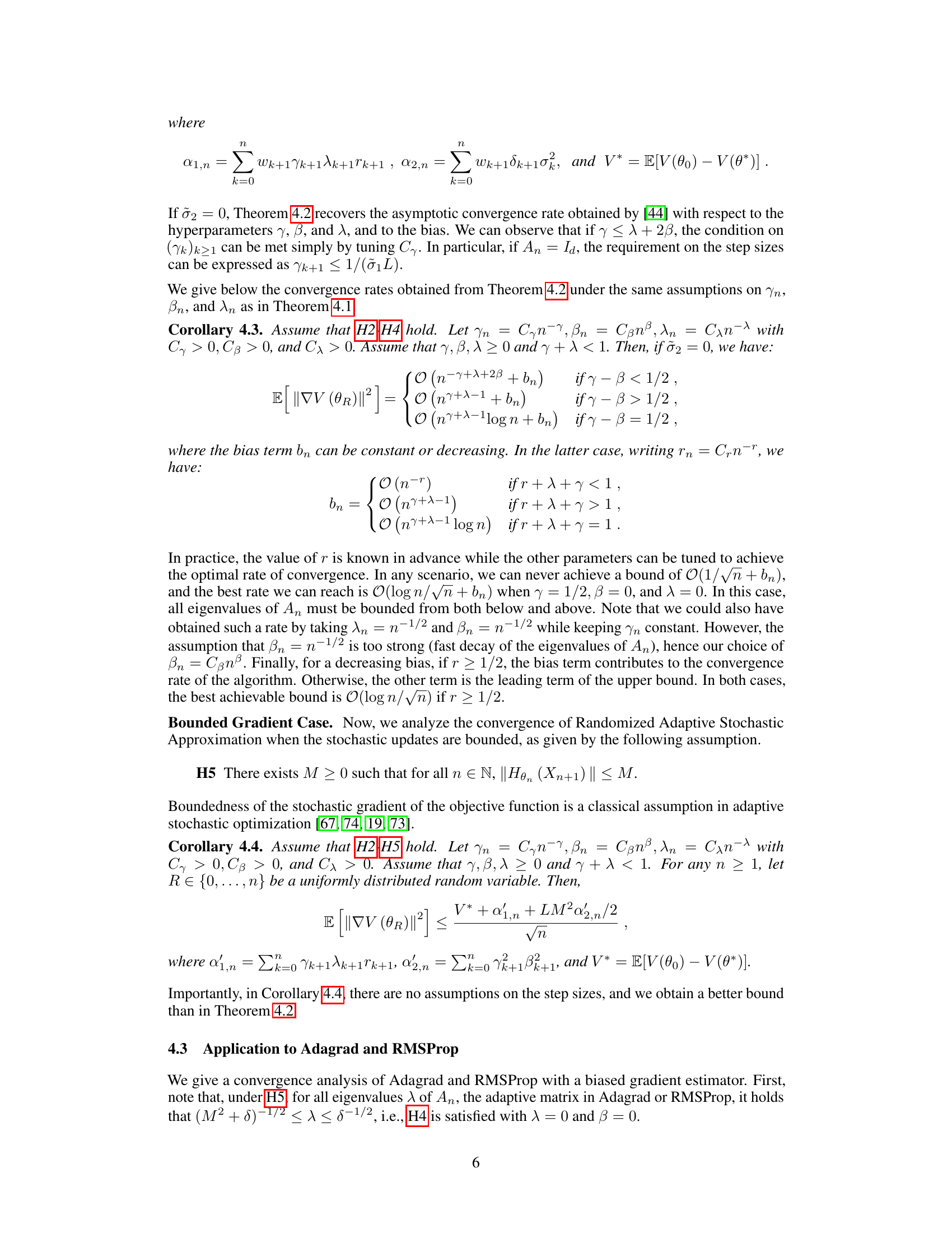
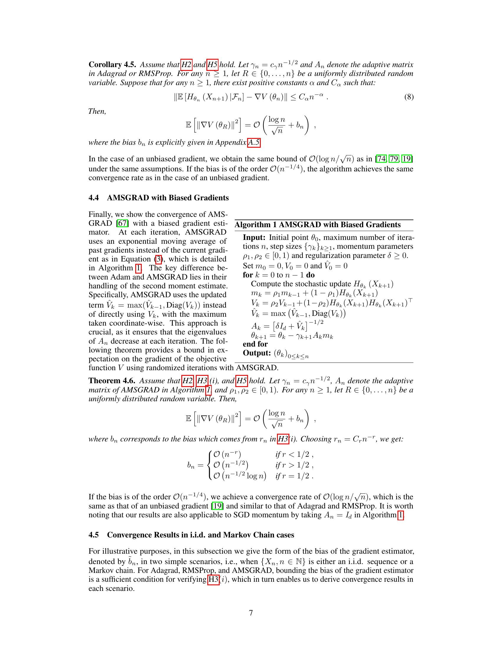
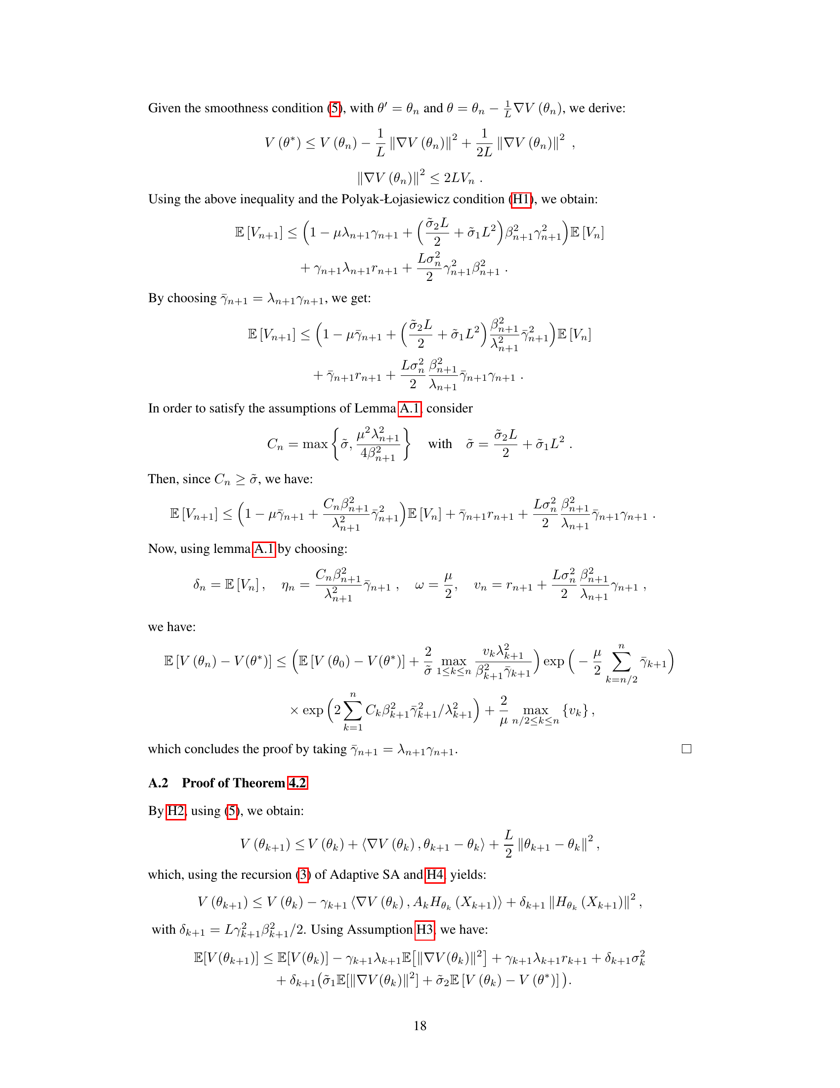
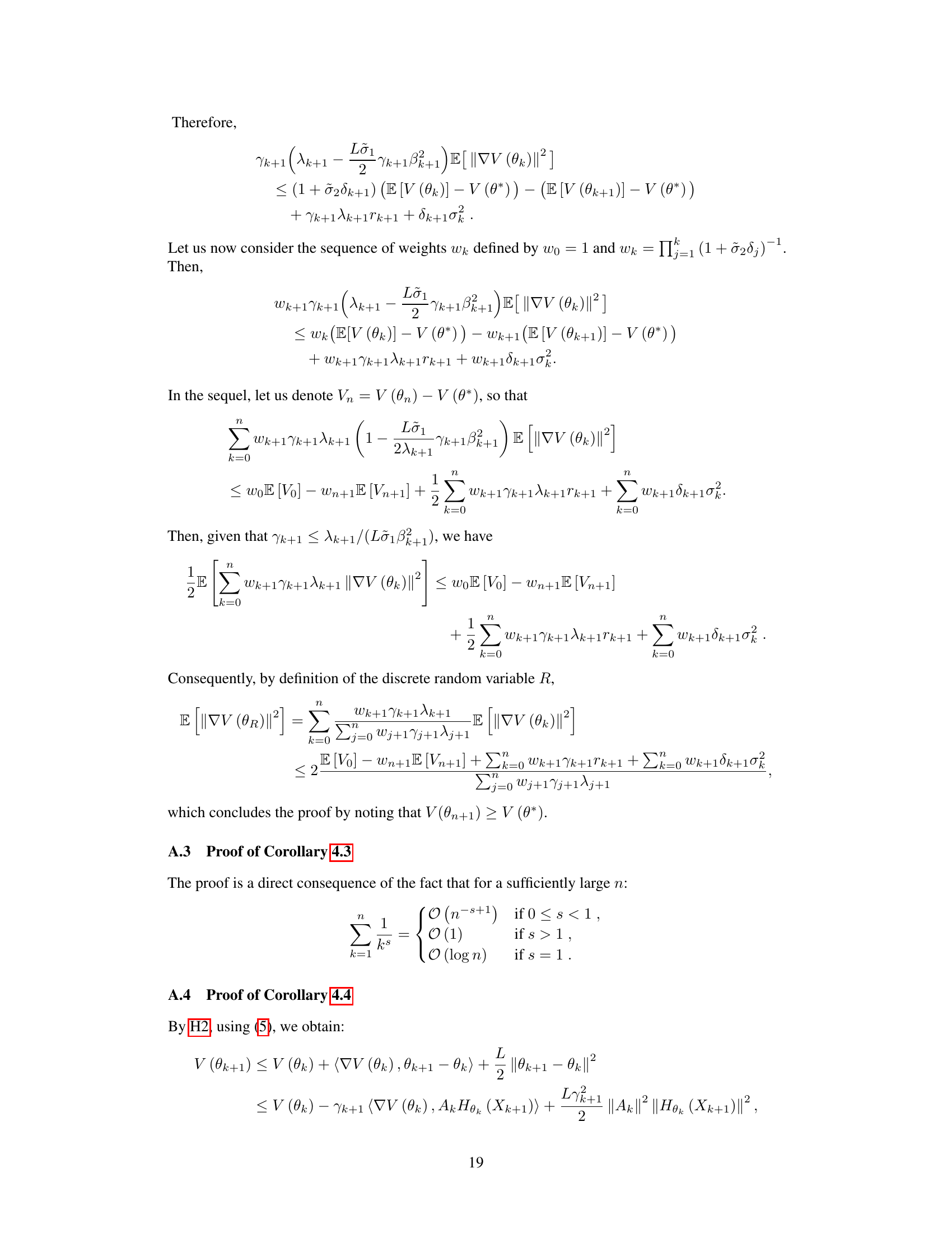
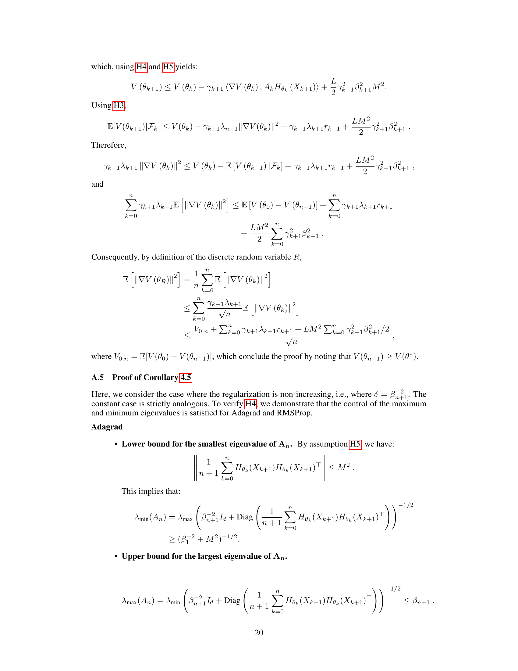
This paper fills this gap by providing a comprehensive non-asymptotic analysis of adaptive SGD with biased gradients. The researchers establish convergence to critical points for smooth non-convex functions under weak assumptions. Importantly, they demonstrate that popular adaptive methods (Adagrad, RMSProp, AMSGrad) maintain similar convergence rates even with biased gradients. The study provides non-asymptotic convergence rate bounds and illustrates the results through several applications with biased gradients, like variational autoencoders. The research also gives insights into how to reduce bias by tuning hyperparameters, making it a significant contribution to both the theoretical and practical aspects of deep learning optimization.
Key Takeaways#
Why does it matter?#
This paper is crucial for researchers working with biased stochastic gradient descent methods, especially in deep learning and reinforcement learning. It provides the first non-asymptotic convergence guarantees for adaptive SGD with biased estimators, bridging a critical gap in the theoretical understanding of widely used optimization algorithms. This work opens avenues for designing more robust and efficient deep learning models.
Visual Insights#

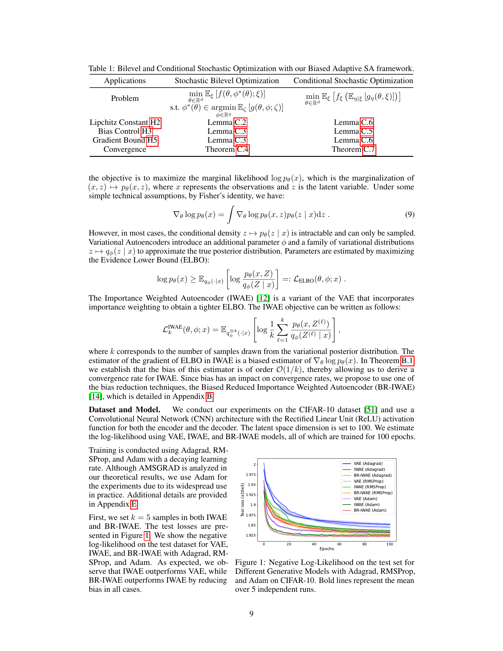
🔼 This figure shows the negative log-likelihood on the CIFAR-10 test set for three generative models (VAE, IWAE, and BR-IWAE) trained using three different optimization algorithms (Adagrad, RMSProp, and Adam). Each model and algorithm combination is represented by a line, with the bold lines indicating the average performance across 5 independent runs. The plot visualizes how the different models and optimization algorithms affect the model’s performance on the test dataset, demonstrating the impact of bias reduction techniques (BR-IWAE) and the choice of optimizer on the final model’s ability to generate realistic data.
read the caption
Figure 1: Negative Log-Likelihood on the test set for Different Generative Models with Adagrad, RMSProp, and Adam on CIFAR-10. Bold lines represent the mean over 5 independent runs.
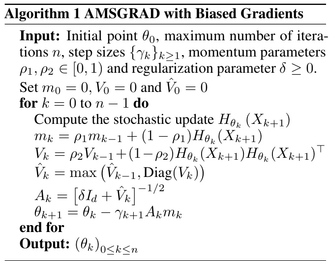
🔼 This table summarizes the applicability of the Biased Adaptive Stochastic Approximation framework to Stochastic Bilevel Optimization and Conditional Stochastic Optimization problems. It shows which assumptions (H2, H3, H5) are satisfied for each problem and the resulting convergence theorems used. It highlights the Lipchitz constant, bias control, gradient bound, and the convergence result for each optimization problem.
read the caption
Table 1: Bilevel and Conditional Stochastic Optimization with our Biased Adaptive SA framework.
In-depth insights#
Biased SGD Analysis#
Analyzing biased stochastic gradient descent (SGD) offers crucial insights into the behavior of optimization algorithms in real-world scenarios where obtaining unbiased gradient estimates is difficult or impossible. A key focus is understanding the impact of bias on convergence rates and the algorithm’s ability to locate critical points, particularly in non-convex settings. Research in this area investigates various types of bias, including time-dependent bias where the bias magnitude changes over iterations and algorithm-specific bias resulting from the approximation techniques used within adaptive step-size methods. Theoretical analyses often involve establishing convergence bounds that consider the magnitude of the bias, highlighting the trade-off between faster convergence and increased bias. Empirical studies using biased SGD in applications like generative adversarial networks and reinforcement learning are vital for validating theoretical findings and demonstrating the algorithm’s effectiveness despite biased gradient estimates. The development of bias-reduction techniques and careful hyperparameter tuning is also critical to mitigate the adverse effects of bias on the optimization process. Such analysis is essential for advancing deep learning theory and practice and improving the robustness and reliability of training procedures.
Adaptive Step Rates#
Adaptive step rate methods in stochastic approximation offer significant advantages over traditional constant step size approaches, particularly in the context of training deep neural networks and other complex models. Their adaptability allows for faster convergence and better handling of non-convex objective functions, where the gradient’s magnitude and direction can vary considerably across the parameter space. This dynamism is crucial because constant step sizes often necessitate meticulous tuning, requiring careful consideration of factors like the learning rate’s decay and initial value, making optimization far from straightforward. Adaptive methods, such as Adagrad, RMSProp, and Adam, automatically adjust the step size based on the past gradients, effectively controlling the learning process and helping overcome the challenges of ill-conditioned problems and saddle points. However, adaptive methods introduce their own complexities. The theoretical analysis of convergence rates becomes significantly more challenging due to the inherent stochasticity and time-dependence of the adaptive steps. Establishing non-asymptotic convergence bounds under weak assumptions requires advanced techniques, often relying on assumptions like Polyak-Lojasiewicz conditions to simplify analysis. Furthermore, practical aspects also need attention, such as the computational overhead of maintaining and updating the adaptive step sizes, and strategies for hyperparameter tuning that leverage the specific properties of the algorithm used and the problem at hand.
Non-Convex Convergence#
Analyzing convergence in non-convex optimization is crucial due to the prevalence of non-convex objective functions in machine learning. Establishing convergence guarantees for non-convex scenarios is significantly more challenging than for convex problems because of the presence of multiple local minima and saddle points. A key focus in such analysis would be establishing conditions under which an optimization algorithm will converge to a stationary point, often a critical point (where the gradient is zero). The analysis often involves techniques from probability theory and stochastic approximation to handle the inherent randomness present in many non-convex optimization algorithms. Convergence rates, indicating how quickly the algorithm approaches a stationary point, are also crucial aspects of non-convex convergence analysis. These rates often depend on several factors including the algorithm’s properties, the problem’s structure (e.g., smoothness, strong convexity properties in certain regions of the space), and the noise level (if the optimization problem is stochastic). Demonstrating convergence in non-convex settings often relies on assumptions about the objective function (e.g., smoothness) and may involve demonstrating that the algorithm avoids undesirable behavior like getting stuck in poor local minima. Ultimately, a comprehensive understanding of non-convex convergence is critical for developing efficient and reliable machine learning algorithms.
IWAE Bias Reduction#
IWAE, or Importance Weighted Autoencoders, presents a powerful approach to variational inference, enhancing the ELBO (Evidence Lower Bound) tightness. However, a significant limitation is the inherent bias in its gradient estimator. This bias stems from the use of Monte Carlo sampling to approximate expectations, leading to inaccurate gradient updates and potentially hindering convergence. Addressing this bias is crucial for reliable model training and improved performance. Several bias reduction techniques have emerged, including the biased reduced IWAE (BR-IWAE), which employs bias reduction techniques such as the BR-SNIS estimator to directly mitigate the effects of bias in the gradient calculation. This method offers an improved trade-off between bias reduction and variance increase compared to naive IWAE. Further research into other bias reduction techniques such as the Jackknife estimator, the Delta method variational inference, or multi-level Monte Carlo methods could also provide promising avenues to enhance IWAE’s accuracy and efficiency, especially for complex models and limited computational resources. Careful consideration of the bias-variance tradeoff is key, as reducing bias too aggressively can lead to increased variance, negating any benefit.
Future Research#
Future research directions stemming from this work could involve extending the theoretical analysis to encompass a broader class of adaptive algorithms and objective functions, moving beyond the current assumptions. A key area to explore is the impact of different adaptive step-size selection strategies on convergence rates, especially in the presence of biased gradients. Investigating alternative bias reduction techniques beyond those presented is crucial for improving convergence. The work could also be extended to explore the application of the biased adaptive framework to specific deep learning tasks such as generative modeling or reinforcement learning, allowing for a more practical evaluation of the theoretical findings. Finally, a deeper exploration into the relationship between the bias and the choice of hyperparameters would further refine practical guidance.
More visual insights#
More on figures

🔼 This figure shows the squared gradient norm (||∇V(θn)||²) for IWAE using Adagrad, RMSProp, and Adam optimizers. The plots are on a logarithmic scale to better visualize the convergence rate. The solid lines represent the average over 5 independent runs, with shaded areas showing variability. Dashed lines indicating theoretical convergence rates are shown only in the left plot (Adagrad). The figure demonstrates how the gradient norm decreases over epochs for each optimizer, illustrating their convergence behavior.
read the caption
Figure 2: Value of ||∇V(θn)||² in IWAE with Adagrad (on the left), RMSProp, and Adam (on the right). Bold lines represent the mean over 5 independent runs. Figures are plotted on a logarithmic scale for better visualization. Both figures have the same scale, so we have not shown the dashed theoretical curves on the right for better clarity.

🔼 This figure displays the results of an experiment using the Adagrad algorithm with varying bias terms (rn) and a learning rate of n⁻¹/². The left panel shows the convergence of the objective function V(θn) towards its minimum V(θ*), while the right panel shows the convergence of the gradient norm ||∇V(θn)||². Different lines represent different bias decay rates (r = 1, 1/4, 1/2, 1, 2, 0), demonstrating the impact of bias on convergence speed. The dashed lines represent the theoretically expected convergence rates of O(n⁻¹/⁴) and O(n⁻¹/²) depending on the bias decay rate.
read the caption
Figure 3: Value of V(θn) – V(θ*) (on the left) and ||∇V(θn)||2 (on the right) with Adagrad for different values of rn = n−r and a learning rate γn = n−1/2. The dashed curve corresponds to the expected convergence rate O(n−1/4) for r = 1/4 and O(n−1/2) for r ≥ 1/2.

🔼 This figure shows the squared gradient norm over epochs for IWAE using three different optimization algorithms: Adagrad, RMSProp, and Adam. The plots are on a logarithmic scale for better visualization, and the solid lines show the mean of 5 independent runs. The dashed lines (only shown on the left plot) represent the theoretical convergence rate.
read the caption
Figure 2: Value of ||∇V(θn)||² in IWAE with Adagrad (on the left), RMSProp, and Adam (on the right). Bold lines represent the mean over 5 independent runs. Figures are plotted on a logarithmic scale for better visualization. Both figures have the same scale, so we have not shown the dashed theoretical curves on the right for better clarity.

🔼 This figure shows the squared gradient norm (||∇V(θn)||²) over epochs for IWAE using three different adaptive algorithms: Adagrad, RMSProp, and Adam. The plots illustrate the convergence rate of the algorithms, with bold lines representing the average over five runs. The logarithmic scale is used for easier visualization of the convergence behavior. The dashed lines (theoretical convergence rates), omitted from the right-hand plots for clarity, would have shown expected convergence rates for different bias values.
read the caption
Figure 2: Value of ||∇V(θn)||² in IWAE with Adagrad (on the left), RMSProp, and Adam (on the right). Bold lines represent the mean over 5 independent runs. Figures are plotted on a logarithmic scale for better visualization. Both figures have the same scale, so we have not shown the dashed theoretical curves on the right for better clarity.

🔼 This figure shows the squared gradient norm for IWAE using Adagrad, RMSProp, and Adam. The plots are on a logarithmic scale to better visualize the convergence rates. Dashed lines representing theoretical convergence rates are only shown in the left plot for clarity.
read the caption
Figure 2: Value of ||∇V(θn)||² in IWAE with Adagrad (on the left), RMSProp, and Adam (on the right). Bold lines represent the mean over 5 independent runs. Figures are plotted on a logarithmic scale for better visualization. Both figures have the same scale, so we have not shown the dashed theoretical curves on the right for better clarity.

🔼 The figure displays the test set negative log-likelihood for three generative models (VAE, IWAE, and BR-IWAE) trained using three different optimization algorithms (Adagrad, RMSProp, and Adam). Each line represents the average performance over five independent runs, with bold lines indicating the mean performance. The graph illustrates the comparative performance of different generative models and optimizers on the CIFAR-10 dataset.
read the caption
Figure 1: Negative Log-Likelihood on the test set for Different Generative Models with Adagrad, RMSProp, and Adam on CIFAR-10. Bold lines represent the mean over 5 independent runs.

🔼 This figure displays the squared gradient norm (||∇V(θn)||²) over epochs for IWAE using three different adaptive optimizers: Adagrad, RMSProp, and Adam. The plots show the mean over 5 independent runs, and use a logarithmic scale for easier visualization. The left panel shows the results for Adagrad, while the right panel shows RMSProp and Adam. Dashed lines representing theoretical convergence rates are included only in the left panel for clarity. The figure illustrates the convergence behavior of these optimizers on the IWAE objective function.
read the caption
Figure 2: Value of ||∇V(θn)||² in IWAE with Adagrad (on the left), RMSProp, and Adam (on the right). Bold lines represent the mean over 5 independent runs. Figures are plotted on a logarithmic scale for better visualization. Both figures have the same scale, so we have not shown the dashed theoretical curves on the right for better clarity.

🔼 This figure shows the impact of the regularization parameter δ on the performance of IWAE using the Adam optimizer on the CIFAR-10 dataset. The test loss (negative log-likelihood) is plotted against the number of epochs for various values of δ (10⁻⁸, 10⁻⁵, 0.001, 0.01, 0.05, 0.1). Each line represents the average of 5 independent runs. The results aim to show how the choice of this regularization parameter affects the convergence rate and overall performance of IWAE with Adam.
read the caption
Figure 9: IWAE on the CIFAR-10 Dataset with Adam for different values of δ. Lines represent the mean over 5 independent runs.

🔼 This figure shows the negative log-likelihood on the CIFAR-10 test set for IWAE using Adagrad and RMSprop optimizers. The x-axis represents the training time in seconds, and the y-axis represents the test loss. Multiple lines are plotted for different values of α (alpha), a hyperparameter that influences the bias of the gradient estimator. The bold lines represent the average test loss over five independent runs; shaded regions indicate variability. The plot shows how the convergence speed of the IWAE algorithm with different optimizers and the values of α.
read the caption
Figure 10: Negative Log-Likelihood on the test set of the CIFAR-10 Dataset for IWAE with Adagrad (on the left) RMSProp (on the right) for Different Values of α over time (in seconds). Bold lines represent the mean over 5 independent runs.
More on tables

🔼 This table summarizes the application of the Biased Adaptive Stochastic Approximation (BSA) framework to Bilevel and Conditional Stochastic Optimization problems. It lists the key assumptions (Lipschitz Constant H2, Bias Control H3, Gradient Bound H5) required for the convergence analysis, and the corresponding lemmas and theorems that prove the convergence rate in each setting. The table allows readers to easily compare the conditions and results for the two different types of problems.
read the caption
Table 1: Bilevel and Conditional Stochastic Optimization with our Biased Adaptive SA framework.

🔼 This table summarizes the assumptions (H2, H3, H5) and convergence results for Stochastic Bilevel Optimization and Conditional Stochastic Optimization using the Biased Adaptive Stochastic Approximation framework proposed in the paper. It shows how the theoretical results apply to these specific applications, indicating which assumptions are satisfied and the corresponding convergence rates (O(log n/√n + bn)). The table highlights the similarities and differences in the application of the framework to these two distinct optimization problems.
read the caption
Table 1: Bilevel and Conditional Stochastic Optimization with our Biased Adaptive SA framework.

🔼 This table presents the negative log-likelihood values achieved on the FashionMNIST test set using various optimization algorithms (SGD, SGD with momentum, Adagrad, RMSProp, and Adam) and different generative models (VAE, IWAE, and BR-IWAE). Lower values indicate better performance. The results demonstrate the relative performance of these methods in this specific setting.
read the caption
Table 3: Comparison of Negative Log-Likelihood on the FashionMNIST Test Set (Lower is Better).
Full paper#

