Lower Bounds of Uniform Stability in Gradient-Based Bilevel Algorithms for Hyperparameter Optimization

↗ OpenReview ↗ NeurIPS Homepage ↗ Chat

TL;DR

#

Key Takeaways

#

Why does it matter?

#

This paper is crucial because it addresses a critical gap in the understanding of gradient-based bilevel optimization algorithms. By establishing tight lower bounds on uniform stability, it offers a more complete picture of algorithm behavior and generalization performance, informing the design and analysis of future algorithms. This is especially relevant given the increasing use of bilevel optimization in various machine learning applications. The results provide general tools for analyzing stability lower bounds in iterative algorithms and validate the limits of uniform stability in characterizing the UD-based algorithm.

Visual Insights

#

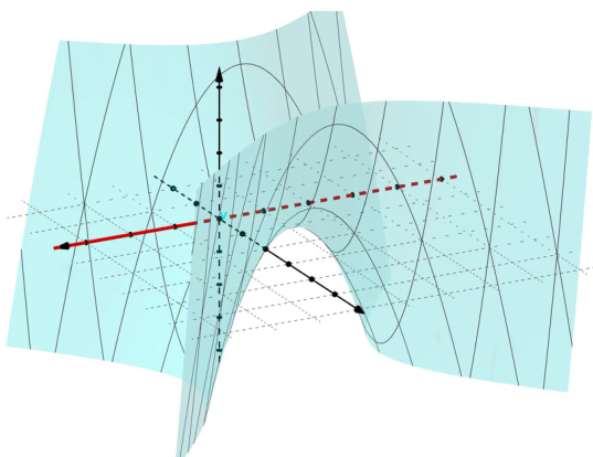
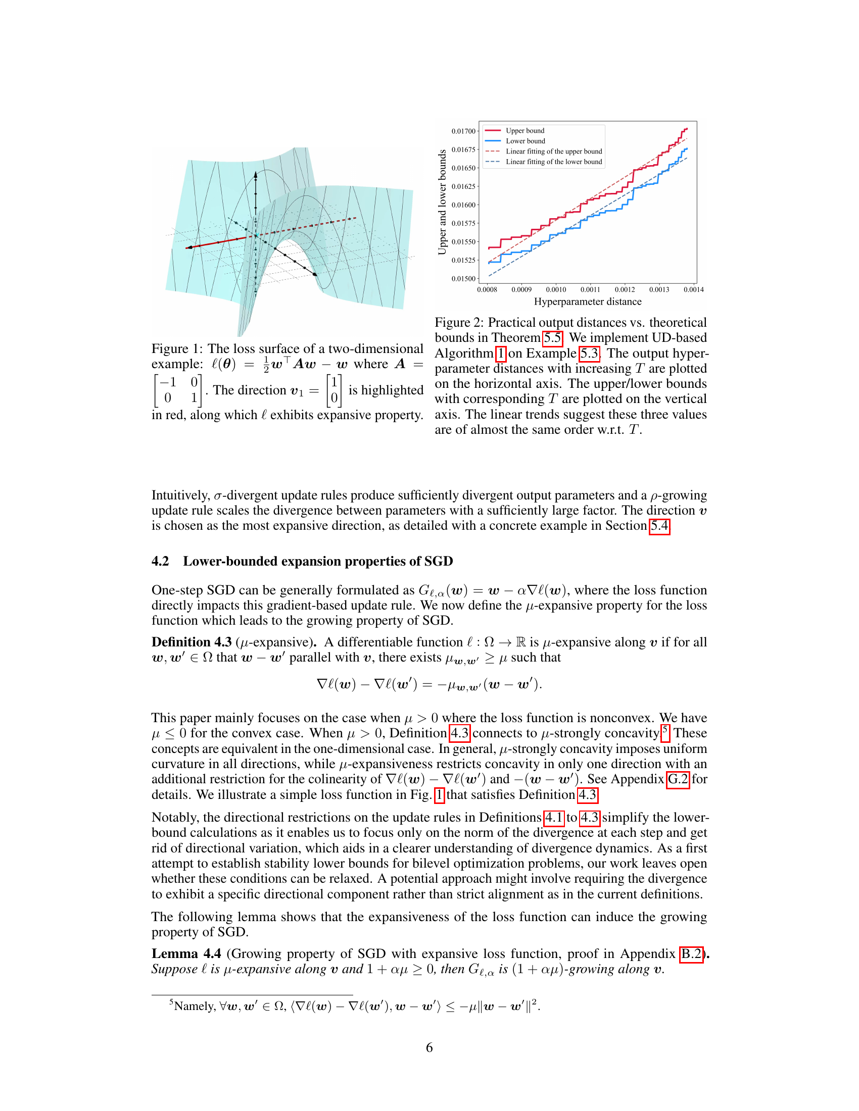
This figure shows a 2D visualization of the loss surface of a function with hyperparameters λ and model parameters θ. The loss function is ℓ(θ) = θTAθ – λθTv1 + λθTv1/2, where A is a symmetric matrix and v1 is a unit eigenvector. The figure highlights the expansive property of the loss function along the direction of v1, which is crucial for establishing lower bounds on algorithmic stability. The figure visually represents the non-convexity of the loss function, showing how it leads to instability in optimization algorithms.

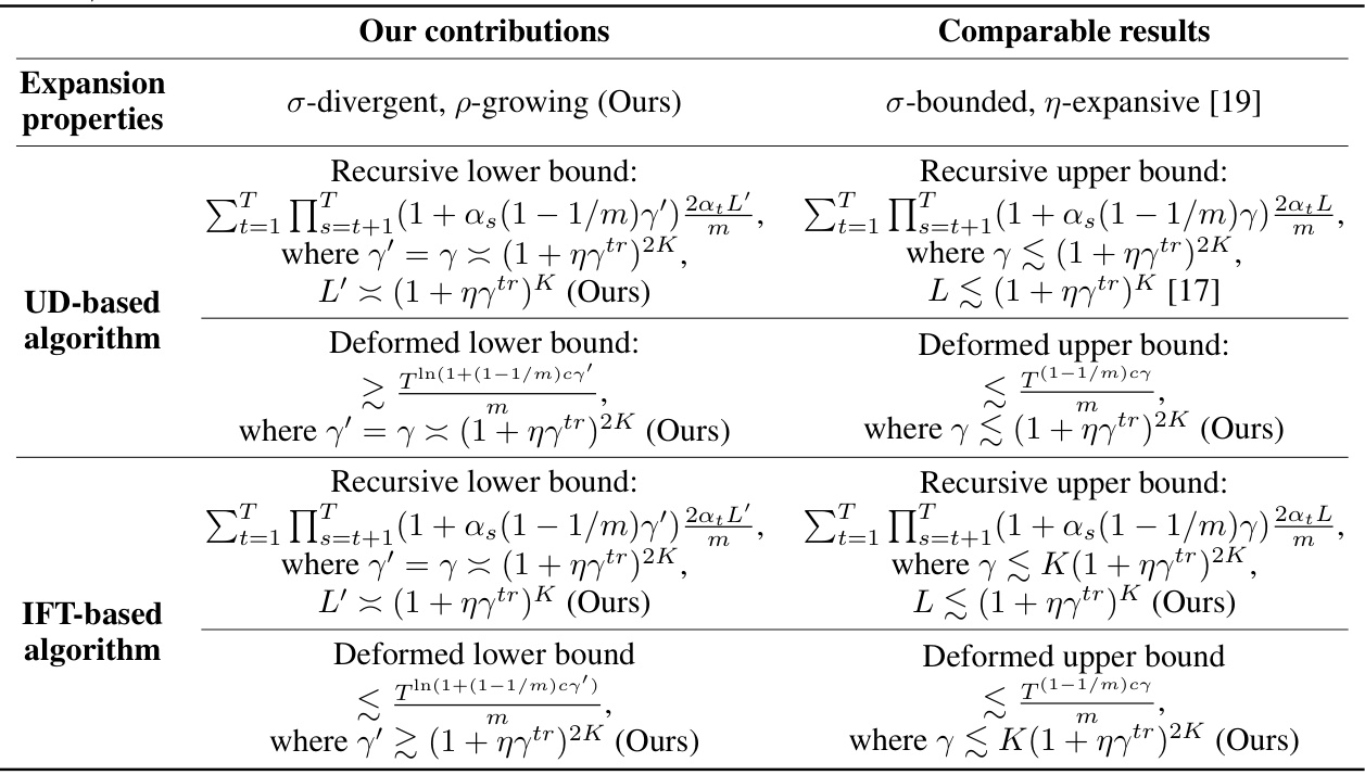
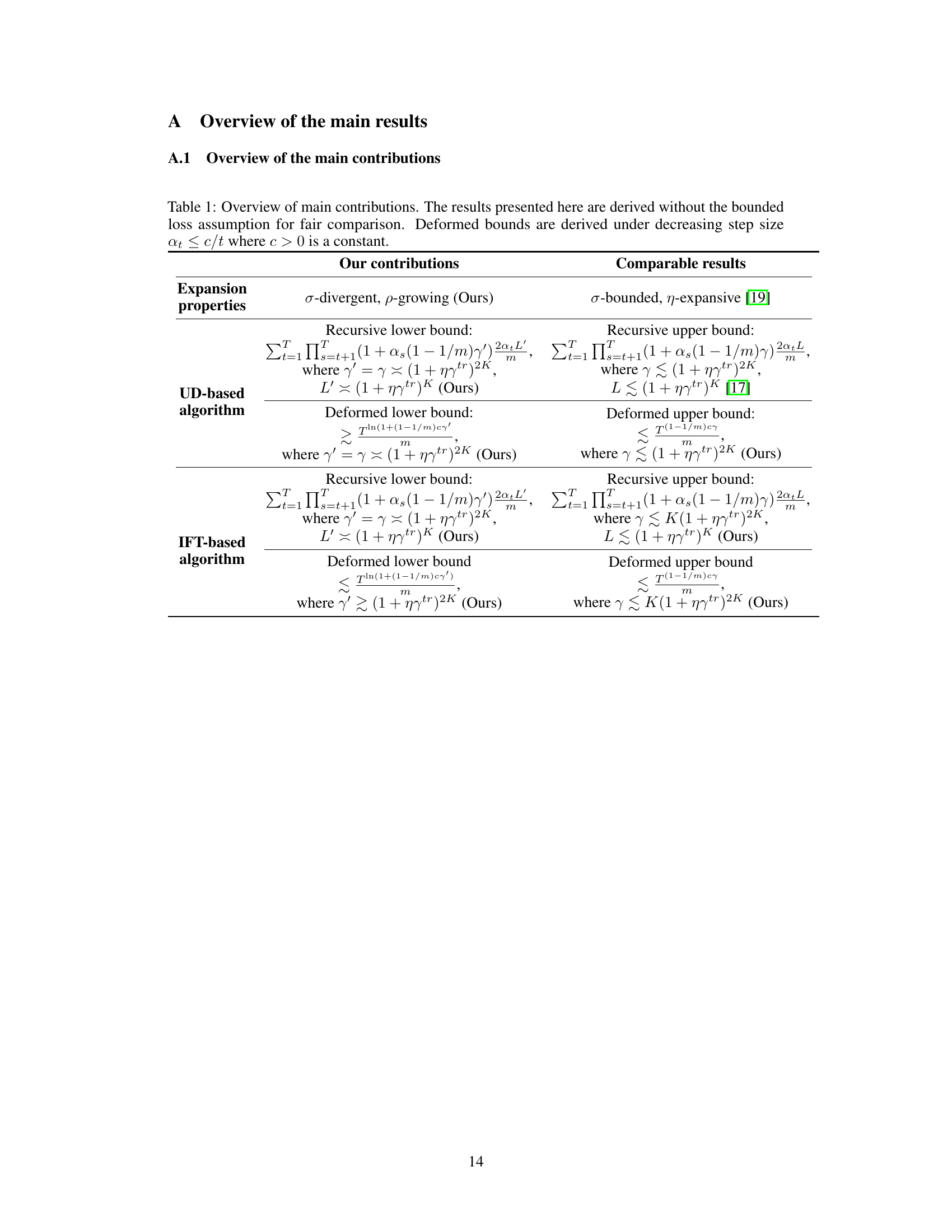
This table summarizes the main contributions of the paper regarding lower and upper bounds on uniform stability for UD-based and IFT-based bilevel optimization algorithms. It compares the authors’ new findings with existing results in the literature. The table shows recursive and deformed lower and upper bounds, highlighting the differences in the key parameters (γ, γ’, L, L’) involved in the stability analysis. It also lists the types of expansion properties used in the analysis.

In-depth insights

#

Bilevel Alg. Stability

#

Analyzing the stability of bilevel algorithms is crucial for understanding their generalization capabilities. Uniform stability, a common measure, quantifies the maximum change in the algorithm’s output when a single training example is altered. However, bilevel optimization’s nested structure presents unique challenges. The outer loop optimizes hyperparameters based on the inner loop’s optimal model parameters. This interdependence makes analyzing stability complex. Researchers often establish upper bounds on uniform stability, but their tightness remains unclear. Lower bounds are essential for determining if these upper bounds are meaningful. Establishing these lower bounds often involves constructing carefully designed examples that highlight the algorithm’s potential instability. The choice of examples and the methods used to analyze these examples are critical, often requiring the introduction of new theoretical tools like lower-bounded expansion properties. The work of establishing tight bounds on bilevel algorithm stability is important for gaining insights into their generalization behavior and improving their design, and shows that, in certain instances, stability analysis may reach its limits.

UD Lower Bounds

#

The heading ‘UD Lower Bounds’ likely refers to a section of a research paper focusing on the theoretical limitations of unrolling-based differentiation (UD) methods in bilevel optimization. The analysis likely involves establishing lower bounds on the algorithm’s uniform stability. This is a significant contribution as it helps determine the inherent limitations of UD and whether existing upper bounds on generalization error are tight. The research probably involves constructing a specific example or family of problems that demonstrates the minimal level of stability achievable by UD-based algorithms. This example would likely have specific properties (e.g., loss function characteristics, hyperparameter structure) designed to expose the algorithm’s vulnerabilities. The analysis might involve a recursive argument, showing that even with carefully chosen parameters, the algorithm’s stability cannot go below a certain value. This would demonstrate the limits of UD, highlighting its potential to overfit and not generalize well in certain situations. Such findings would be valuable for understanding the trade-offs involved in using UD, guiding future research towards algorithms with improved stability or alternative bilevel optimization techniques. The study may also compare the lower bounds with existing upper bounds to determine the tightness of previous analyses.

IFT-Based Analysis

#

An IFT-based analysis of a bilevel optimization algorithm would delve into the algorithm’s theoretical properties using the Implicit Function Theorem. This theorem allows for analyzing the sensitivity of the inner optimization problem’s solution to changes in the outer-level hyperparameters. A key aspect would be deriving the hypergradient, which represents the gradient of the validation or testing loss with respect to the hyperparameters. The derivation would likely involve careful consideration of the implicit differentiation implied by the inner optimization. This analysis is important because it provides insights into the algorithm’s convergence behavior and generalization capabilities, especially in the context of hyperparameter optimization (HPO). The analysis might involve making assumptions, for example, about the differentiability of the loss function and the regularity conditions of the inner problem’s solution, to ensure the applicability of the Implicit Function Theorem. The results would potentially yield insights into the tightness of existing generalization bounds derived using algorithmic stability or other generalization theories. The analysis might also assess the computational cost of this approach, comparing it to methods based on unrolling differentiation, which directly computes the hypergradient via backpropagation. Such a comparison could reveal trade-offs between computational complexity and the precision of the hypergradient approximation. Finally, the IFT-based analysis could be used to inform the design of improved bilevel optimization algorithms with better convergence properties and generalization performance. Ultimately, a comprehensive IFT-based analysis offers a valuable theoretical lens to investigate the behavior of bilevel optimization algorithms for hyperparameter optimization, complementing the empirical studies and providing a rigorous foundation for understanding their performance and properties.

Expansion Properties

#

The concept of “Expansion Properties” in the context of a research paper likely revolves around characterizing how certain operations or updates amplify differences in the system’s state. This is crucial for analyzing the behavior of iterative algorithms, especially in scenarios involving hyperparameter optimization or gradient descent. The core idea is to mathematically formalize how small initial variations can lead to significant divergence in later iterations. This divergence, often undesirable, can be analyzed by defining properties that quantify this expansion. For example, a specific property might guarantee that the distance between two sequences of updates grows at least by a certain factor at each iteration, thus characterizing the expansion’s magnitude. These properties are valuable tools; they help establish lower bounds on the stability of algorithms, providing insights into how unstable an algorithm can potentially be. Moreover, expansion properties act as bridges between the analysis of stability (how much the algorithm output changes due to small perturbations) and the algorithm’s inherent behavior. By establishing these properties, researchers can gain a deeper understanding of the relationship between an algorithm’s update rules and its overall performance, leading to more robust and efficient algorithm designs.

Future Research

#

Future research directions stemming from this work could explore several promising avenues. Extending the theoretical framework to encompass non-smooth loss functions is crucial, as many real-world machine learning problems involve non-smooth objectives. Furthermore, investigating the tightness of stability bounds for other bilevel optimization algorithms, beyond the UD- and IFT-based methods analyzed here, would provide a more comprehensive understanding of their generalization capabilities. Developing techniques to directly analyze the generalization error, rather than relying solely on algorithmic stability, would offer a more direct assessment of algorithm performance. This could involve novel approaches combining empirical risk minimization with stability analysis. Finally, empirical validation of the theoretical findings through comprehensive simulations and experiments on diverse datasets is essential to confirm the practical implications of the theoretical bounds, and to explore the impact of hyperparameter choices on algorithmic behavior.

More visual insights

#

More on figures

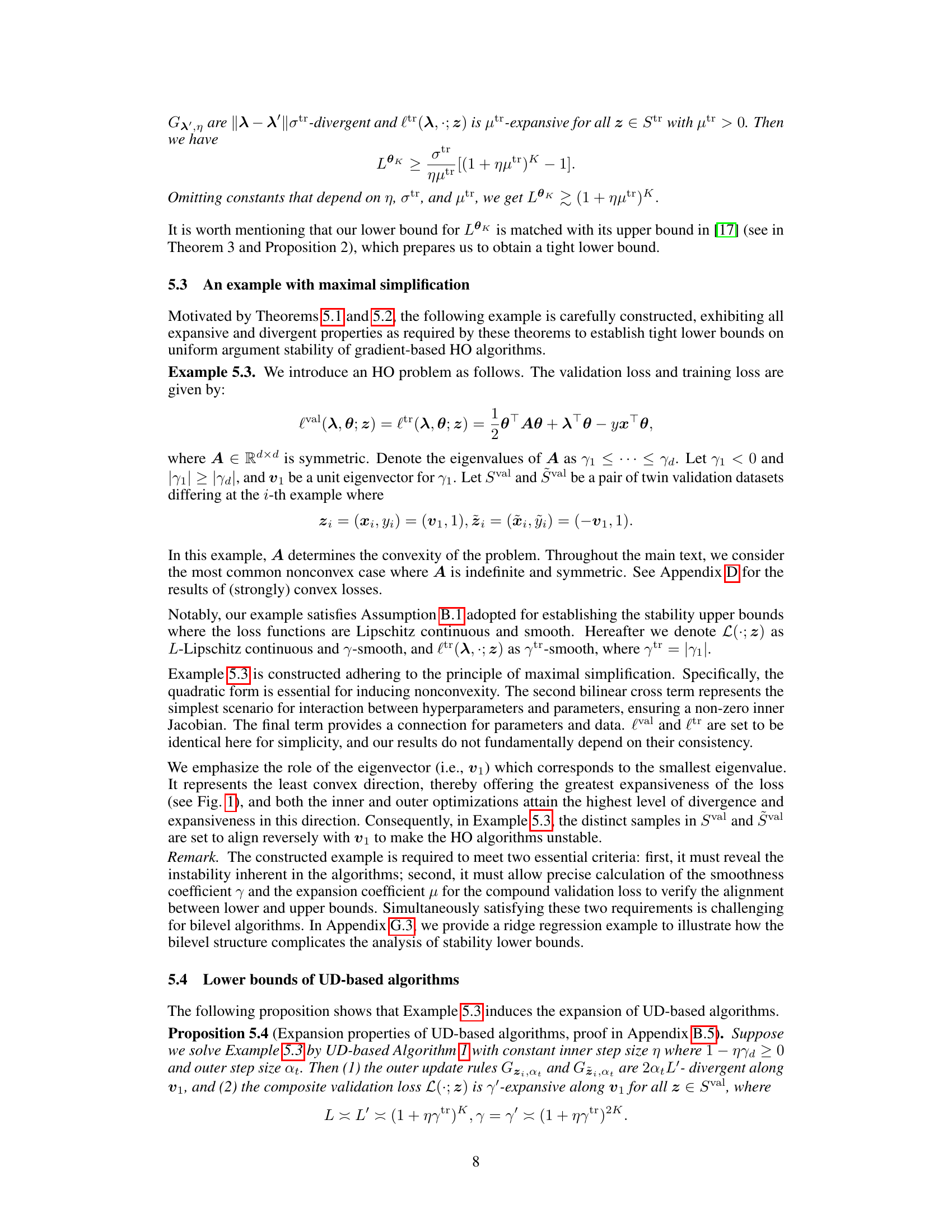
This figure compares practical results from running UD-based Algorithm 1 on a specific example (Example 5.3) with theoretical upper and lower bounds derived in Theorem 5.5. The x-axis represents the distance between hyperparameters at different iterations (T), while the y-axis shows the corresponding upper and lower bounds for the uniform argument stability. The linear relationship between practical and theoretical values in the graph suggests that the upper bounds established in prior work are tight.

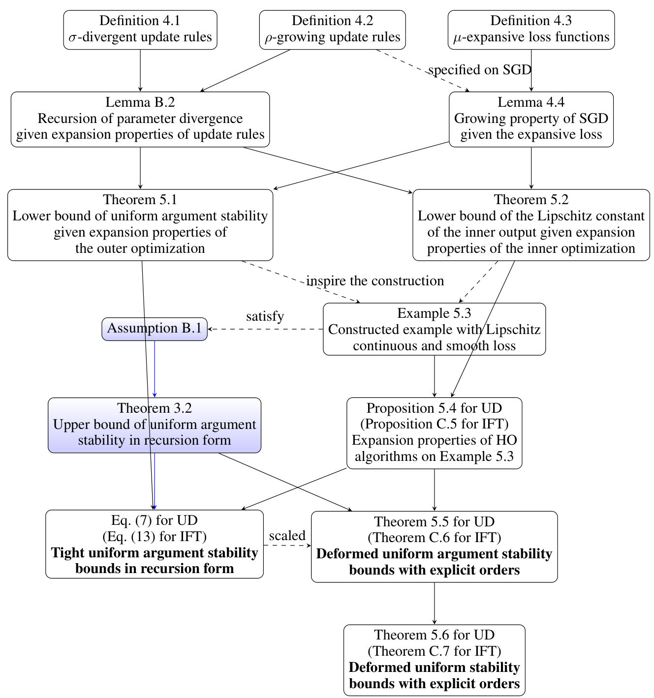
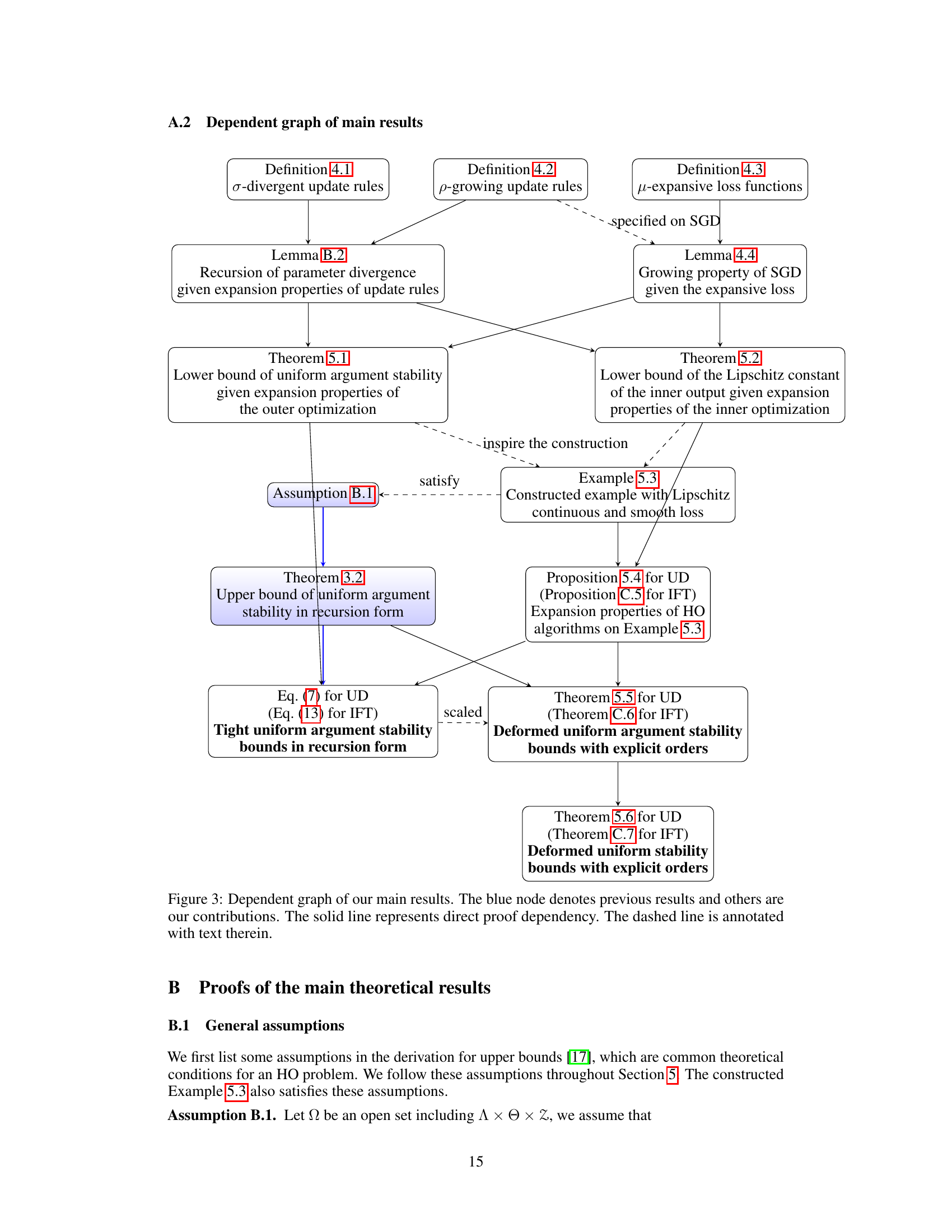
This figure shows the dependencies between the different theorems and lemmas in the paper. The blue nodes represent pre-existing results from other works, while the other nodes represent the novel contributions of this paper. Solid lines indicate direct dependencies (e.g., Theorem 5.1 directly depends on Lemma B.2), while dashed lines highlight indirect influences or supporting arguments. The figure visually summarizes the logical flow and relationships between the key concepts and findings presented in the paper.

This figure compares the practical output hyperparameter distances of the UD-based algorithm (Algorithm 1) on Example 5.3 against the theoretical upper and lower bounds derived in Theorem 5.5. The horizontal axis represents the number of outer iterations (T), while the vertical axis shows the distance between the hyperparameters obtained from two twin validation sets. The plot visually demonstrates that the practical distances closely align with the theoretical bounds, exhibiting a similar linear trend with respect to T, thus supporting the claim that the theoretical bounds are tight.

This figure shows the results of a practical experiment validating the theoretical bounds derived in Theorem 5.5 of the paper. The UD-based algorithm (Algorithm 1) is applied to Example 5.3, and the hyperparameter distance between the outputs for different numbers of iterations (T) is measured. The plot compares these actual distances to the theoretical upper and lower bounds calculated using the formulas in Theorem 5.5. The close alignment and similar linear trends of the practical results and theoretical bounds demonstrate the tightness of the theoretical analysis for the UD-based algorithm.

This figure compares the practical hyperparameter distances obtained from running the UD-based Algorithm 1 with the theoretical upper and lower bounds derived in Theorem 5.5. The x-axis shows the hyperparameter distance, while the y-axis represents the theoretical bounds. The linear trends observed suggest a strong agreement between the practical results and theoretical bounds, indicating the tightness of the analysis.

This figure compares the practical output hyperparameter distances against the theoretical upper and lower bounds derived in Theorem 5.5. The UD-based Algorithm 1 is applied to Example 5.3, and the results show that practical distances and theoretical bounds exhibit similar linear trends, indicating that the bounds tightly characterize the stability.

Full paper

#