TL;DR#
Temporal graph learning is crucial but faces challenges with existing methods like RNNs (long-range dependencies) and Transformers (high complexity). Current approaches often treat temporal graphs as sequences of static snapshots, neglecting the continuous evolution of the underlying graph structure. This can result in inefficient modeling and suboptimal performance.
This paper proposes GRAPHSSM, a novel framework that uses state space models (SSMs) to directly model the continuous-time dynamics of temporal graphs. By integrating structural information via Laplacian regularization, it overcomes the limitations of sequence-based models. GRAPHSSM shows improved performance compared to existing approaches across various benchmarks, demonstrating its effectiveness in capturing long-range dependencies and handling large-scale graphs efficiently.
Key Takeaways#
Why does it matter?#
This paper is crucial for researchers in temporal graph learning due to its novel approach using state space models. It addresses the limitations of existing methods like RNNs and Transformers in handling long-range dependencies and high computational complexity by introducing a new framework, GRAPHSSM. This opens up new avenues for research in handling dynamic graph data, leading to improved performance in various applications like social network analysis, traffic prediction, and financial modeling. The principled approach, theoretical analysis, and extensive experimental results make this paper highly impactful and relevant to current research trends.
Visual Insights#

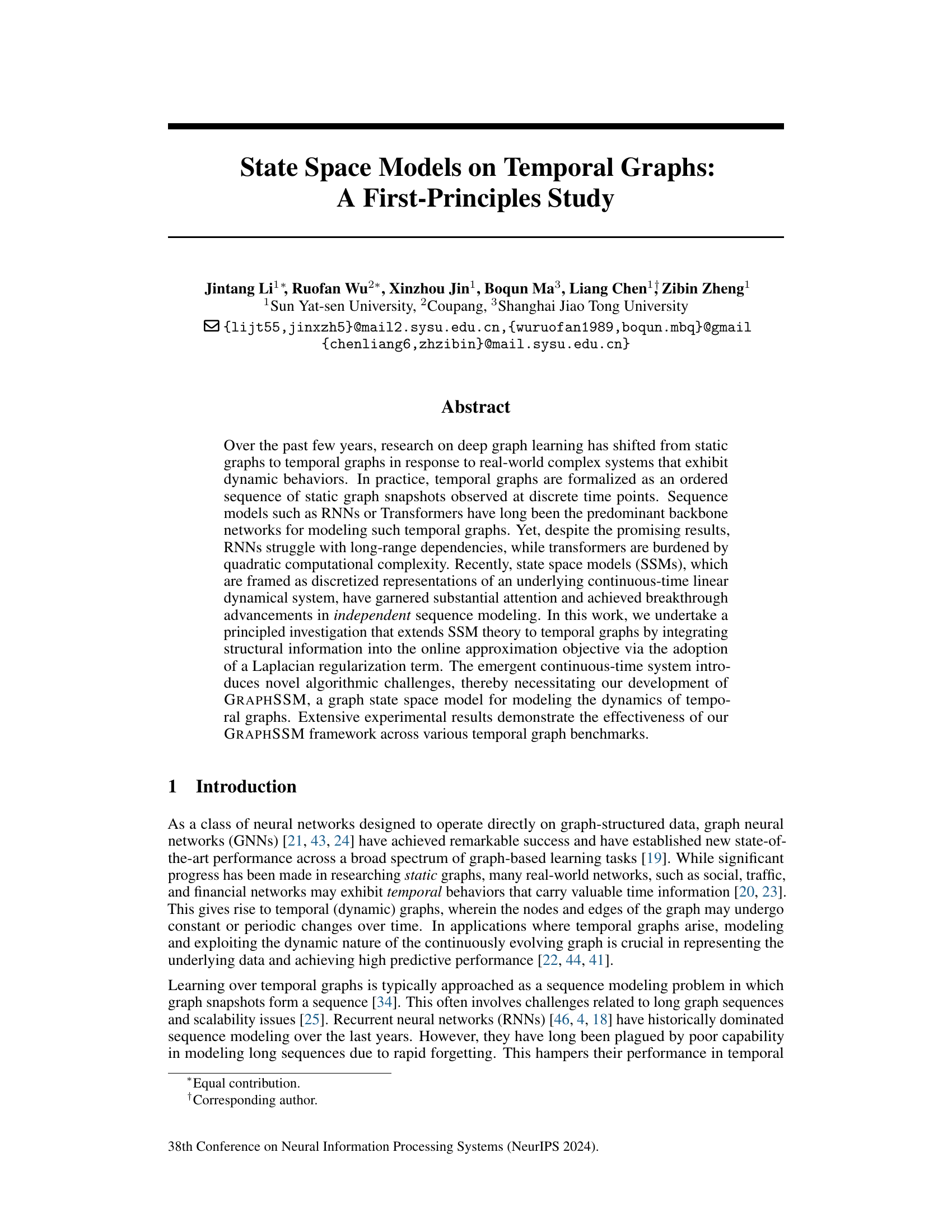
🔼 The figure illustrates the GRAPHSSM framework, which is a state space model for temporal graphs. The framework consists of multiple blocks, each containing a graph convolution layer, an SSM layer, and a residual connection. The input is a sequence of graph snapshots, and the output is a prediction of some property of the graph.
read the caption
Figure 1: GRAPHSSM framework.

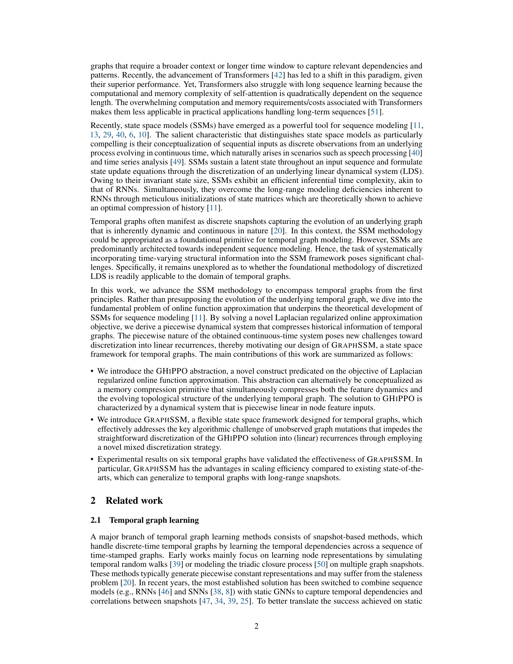
🔼 This table compares four different neural network architectures commonly used for sequence modeling: RNNs, SNNs, Transformers, and SSMs. For each architecture, it provides a qualitative assessment of training speed, inference speed, the number of parameters, overall performance, and limitations.
read the caption
Table 1: Comparisons of different neural network architectures for sequence modeling.
In-depth insights#
Temporal Graph SSMs#
Temporal Graph State Space Models (SSMs) represent a powerful advancement in handling dynamic graph data. Traditional sequence models like RNNs and Transformers struggle with the complexities of temporal dependencies and computational costs associated with large graphs. SSMs offer an elegant solution by framing the temporal graph as a discretized representation of an underlying continuous-time system. This approach allows for efficient modeling of long-range dependencies, which are often problematic for other methods. The key challenge lies in incorporating the inherent structural information of the graph into the SSM framework. This typically involves integrating graph-specific operators (like Laplacian regularization) into the model’s objective function, which necessitates novel algorithmic solutions for efficient online approximation and discretization. The resulting models are often piecewise linear, reflecting the dynamic nature of edge additions and deletions. This piecewise property introduces additional complexities in the discretization process, necessitating methods to handle unobserved mutations. Overall, Temporal Graph SSMs present a promising research direction offering efficiency and scalability advantages over existing methods, though careful consideration of discretization and handling of unobserved changes remains crucial for robust performance.
GHIPPO Abstraction#
The GHIPPO abstraction, a core contribution of the paper, extends the HIPPO framework to temporal graphs. It frames the problem of continuous-time dynamic modeling as an online function approximation task, moving beyond independent sequence modeling to integrate the evolving graph structure. This is achieved by incorporating a Laplacian regularization term into the objective function, encouraging smoothness of memory compression across interconnected nodes. The resulting dynamical system is piecewise linear, capturing both feature dynamics and topological changes, but this piecewise nature introduces subsequent algorithmic challenges for discretization. The key innovation lies in effectively compressing both feature and structural information simultaneously, unlike prior SSM approaches that primarily focus on individual sequences, representing a significant step toward truly understanding temporal graph dynamics. The Laplacian regularization elegantly incorporates the graph structure, making GHIPPO a principled approach for temporal graph modeling.
GRAPHSSM Framework#
The GRAPHSSM framework, a novel approach for modeling temporal graph dynamics, integrates state-space models (SSMs) with graph neural networks (GNNs). Its core innovation lies in the GHIPPO abstraction, which efficiently compresses historical information from temporal graphs through a Laplacian regularized online function approximation. Unlike traditional SSMs primarily designed for independent sequences, GRAPHSSM directly incorporates the graph’s evolving structure. The framework introduces a piecewise dynamical system, efficiently addressing the challenges of unobserved graph mutations using a mixed discretization strategy, combining GNNs with novel node feature and representation mixing mechanisms. GRAPHSSM’s design enables scalable and efficient handling of long temporal sequences with impressive empirical results surpassing existing baselines on various benchmarks. The framework is highly flexible, accommodating different SSM architectures (S4, S5, S6) with choices for mixing strategies and initialization techniques to optimize performance for different datasets.
Mixed Discretization#
The core challenge addressed by ‘Mixed Discretization’ is how to effectively handle unobserved graph mutations when discretizing the continuous-time dynamics of temporal graphs. Standard discretization methods fail because they assume continuous observations, while in reality, the underlying graph structure changes between observed snapshots. The solution proposed involves a mixed discretization strategy that combines two approaches: inter-node mixing (approximating diffusion among nodes using graph neural networks) and intra-node mixing (combining features from consecutive snapshots). This approach cleverly addresses the lack of observed graph mutations by leveraging the relational structure inherent in temporal graphs. The inter-node mixing step incorporates connectivity information to approximate the continuous evolution while intra-node mixing uses a learned mechanism to blend information from adjacent snapshots. This approach’s effectiveness is supported by empirical results showing enhanced performance, making it a significant contribution to the field. The piecewise continuous time nature of the underlying dynamics poses a challenge, but mixed discretization effectively bridges the gap between continuous theory and discrete observations.
Future Extensions#
The research paper’s ‘Future Extensions’ section could explore several promising avenues. Extending the GHIPPO framework to handle continuous-time temporal graphs (CTTGs) is crucial, as current methods struggle with the inherent continuous nature of many real-world networks. This would require addressing the challenges of unobserved mutations and developing robust discretization techniques beyond piecewise linear approximations. Investigating alternative memory compression schemes that facilitate smoother dynamical systems, possibly through modified Laplacian regularizations or objective functions, is another key area. Furthermore, research into more sophisticated mixing mechanisms to better approximate unobserved dynamics between discrete snapshots would significantly improve accuracy. Finally, exploring the applicability of GRAPHSSM to different types of graph neural networks (GNNs) and evaluating its performance on a wider range of benchmarks would enhance the framework’s generalizability and establish its practical effectiveness.
More visual insights#
More on figures

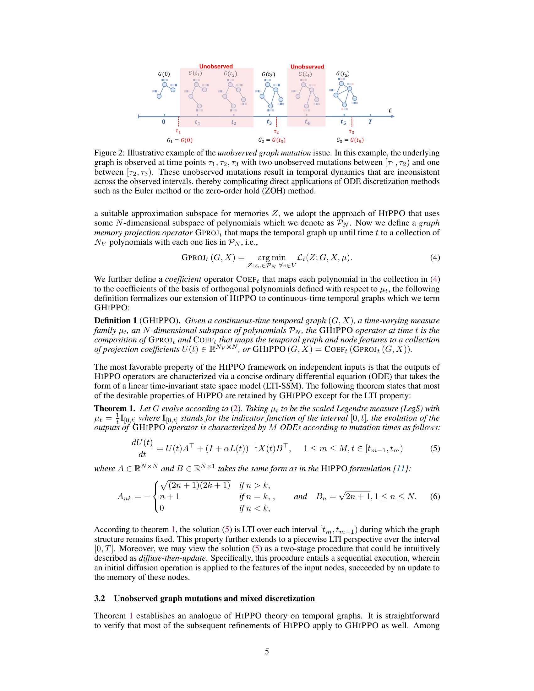
🔼 This figure illustrates the problem of unobserved graph mutations in temporal graphs. The underlying graph changes at times t₁, t₂, t₄, and t₅, but these changes are not observed directly. Instead, only snapshots of the graph are observed at times τ₁, τ₂, and τ₃. These unobserved mutations make it difficult to model the continuous-time evolution of the graph using standard ODE discretization methods.
read the caption
Figure 2: Illustrative example of the unobserved graph mutation issue. In this example, the underlying graph is observed at time points τ₁, τ₂, τ₃ with two unobserved mutations between [τ₁, τ₂) and one between [τ₂, τ₃). These unobserved mutations result in temporal dynamics that are inconsistent across the observed intervals, thereby complicating direct applications of ODE discretization methods such as the Euler method or the zero-order hold (ZOH) method.

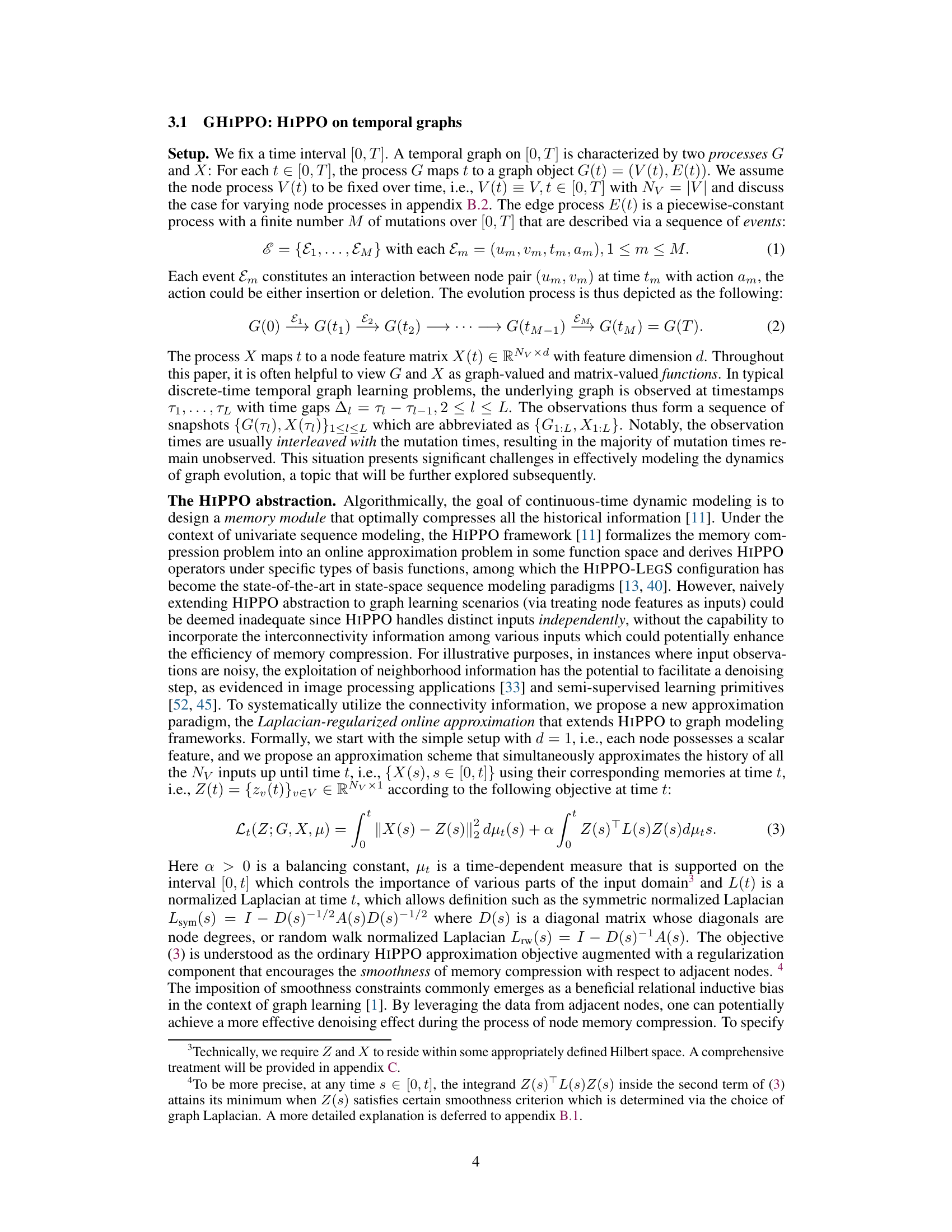
🔼 This figure compares the performance of GRAPHSSM using three different initialization strategies for the A matrix: HIPPO, Random, and Constant. The results are shown for four different datasets: DBLP-3, Brain, Reddit, and DBLP-10. The y-axis represents the Micro-F1 score (%), a measure of the model’s performance. The figure illustrates that the HIPPO initialization strategy consistently outperforms the other two, suggesting it is a more effective approach for this task.
read the caption
Figure 3: Comparison of GRAPHSSM with different initialization strategies.
More on tables

🔼 This table presents the performance comparison of various node classification methods on four small-scale temporal graphs (DBLP-3, Brain, Reddit, DBLP-10). The results are reported using Micro-F1 and Macro-F1 scores, with the best and second-best performances highlighted for each dataset. The table allows for a direct comparison of GRAPHSSM against several established baselines, including static graph embedding methods, temporal graph embedding methods, and temporal graph neural networks.
read the caption
Table 2: Node classification performance (%) on four small scale temporal graphs. The best and the second best results are highlighted as red and blue, respectively.
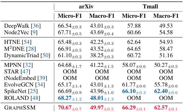
🔼 This table compares the performance of various methods on two large-scale temporal graph datasets (arXiv and Tmall) in terms of Micro-F1 and Macro-F1 scores for node classification. It highlights the scalability challenges faced by some methods, indicated by ‘OOM’ (out of memory) entries, showcasing GRAPHSSM’s superior performance on large, long-range temporal graph datasets.
read the caption
Table 3: Node classification performance (%) on large scale temporal graphs. OOM: out-of-memory.

🔼 This table presents the performance comparison of different methods on four small-scale temporal graph datasets (DBLP-3, Brain, Reddit, DBLP-10) in terms of node classification. The metrics used are Micro-F1 and Macro-F1 scores. The best and second-best results for each metric and dataset are highlighted in red and blue, respectively. The table shows that the proposed GRAPHSSM method outperforms other methods on most datasets.
read the caption
Table 2: Node classification performance (%) on four small scale temporal graphs. The best and the second best results are highlighted as red and blue, respectively.

🔼 This table presents the ablation study results on the impact of different mixing mechanisms used in the GRAPHSSM-S4 model. It compares the performance (Micro-F1 and Macro-F1 scores) of four configurations: no mixing, feature mixing only in the first layer, representation mixing only in the first layer, and representation mixing in the second layer. The results are presented for four different datasets: DBLP-3, Brain, Reddit, and DBLP-10.
read the caption
Table 5: Ablation results (%) of GRAPHSSM-S4 with different mixing configurations.

🔼 This table presents the performance comparison of different methods on four small-scale temporal graph datasets (DBLP-3, Brain, Reddit, DBLP-10) in terms of node classification. The metrics used are Micro-F1 and Macro-F1 scores, representing the average F1 score across all classes and the macro-averaged F1 score, respectively. The best and second-best results for each dataset are highlighted for easy comparison. The table includes both static graph embedding methods and temporal graph neural network methods.
read the caption
Table 2: Node classification performance (%) on four small scale temporal graphs. The best and the second best results are highlighted as red and blue, respectively.
Full paper#
