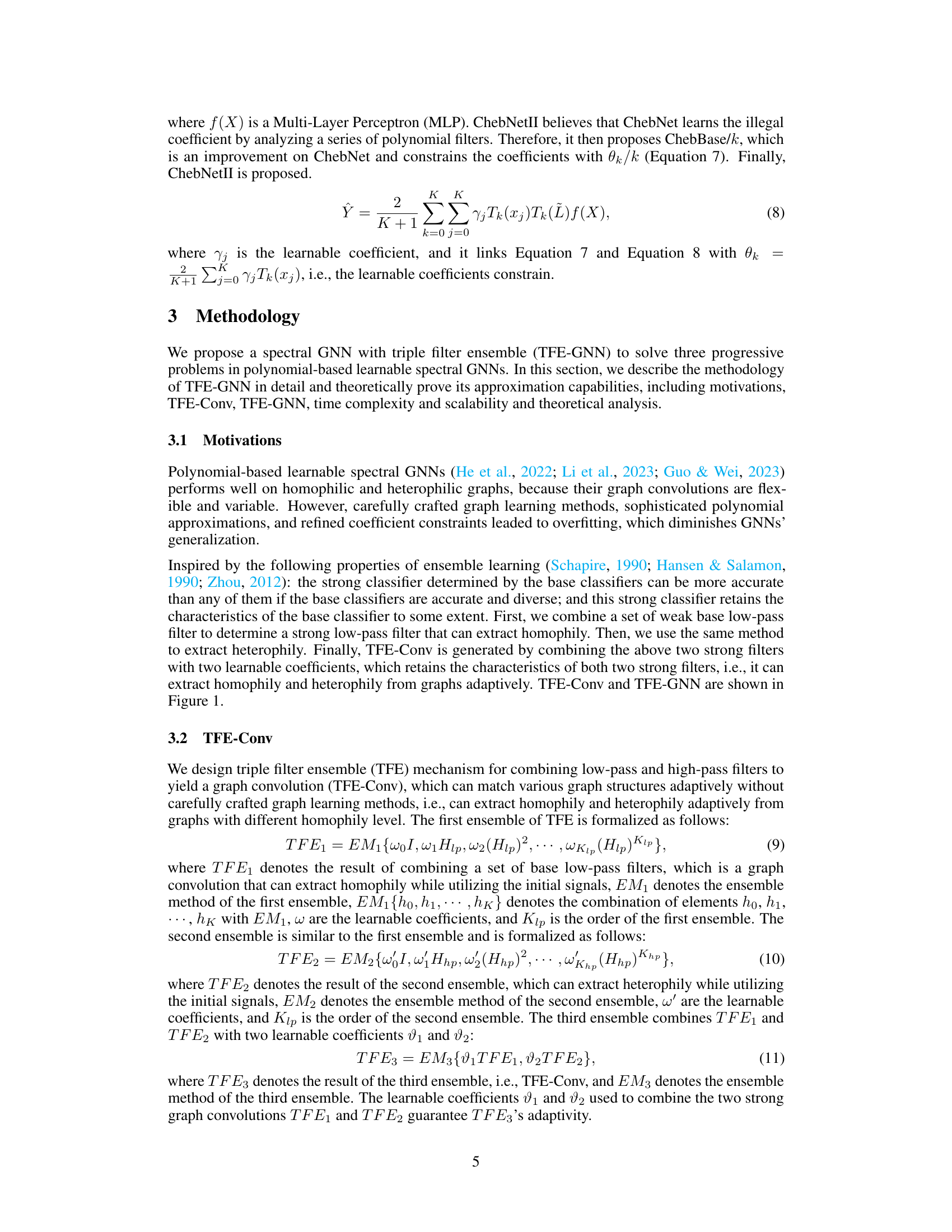
↗ OpenReview ↗ NeurIPS Homepage ↗ Chat
TL;DR#
Polynomial-based learnable spectral GNNs have shown promise but suffer from three key issues: real-world performance lagging behind theoretical approximation abilities, overfitting due to complex learning methods and constraints, and difficulty in handling both homophily and heterophily. These problems hinder the generalization and robustness of existing models.
This research introduces TFE-GNN, a novel spectral GNN that addresses these issues. TFE-GNN employs a triple filter ensemble mechanism to adaptively extract homophily and heterophily, avoiding complex constraints and enhancing generalization. Experimental results show it outperforms other state-of-the-art GNNs on various real-world datasets, proving the effectiveness of the proposed method.
Key Takeaways#
Why does it matter?#
This paper is crucial because it addresses the limitations of existing spectral graph neural networks (GNNs) by proposing a novel Triple Filter Ensemble (TFE) mechanism. This innovative approach enhances model generalization, improves performance on real-world datasets, and offers a new perspective on the combination of homophily and heterophily in GNNs, which is highly relevant to ongoing research in graph machine learning. It provides a new state-of-the-art model (TFE-GNN) and lays the groundwork for future investigations into more effective and robust GNN architectures.
Visual Insights#
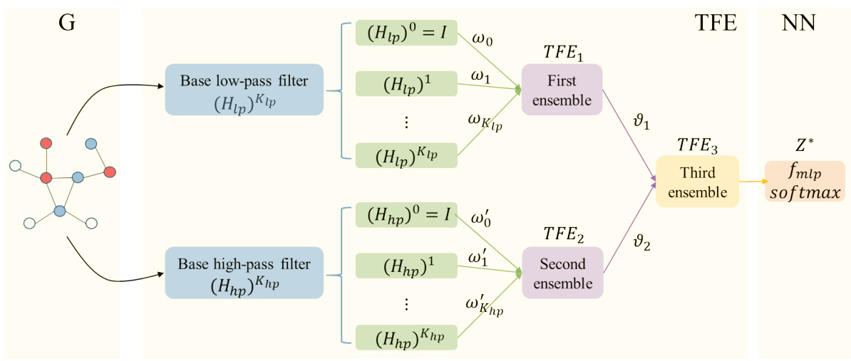
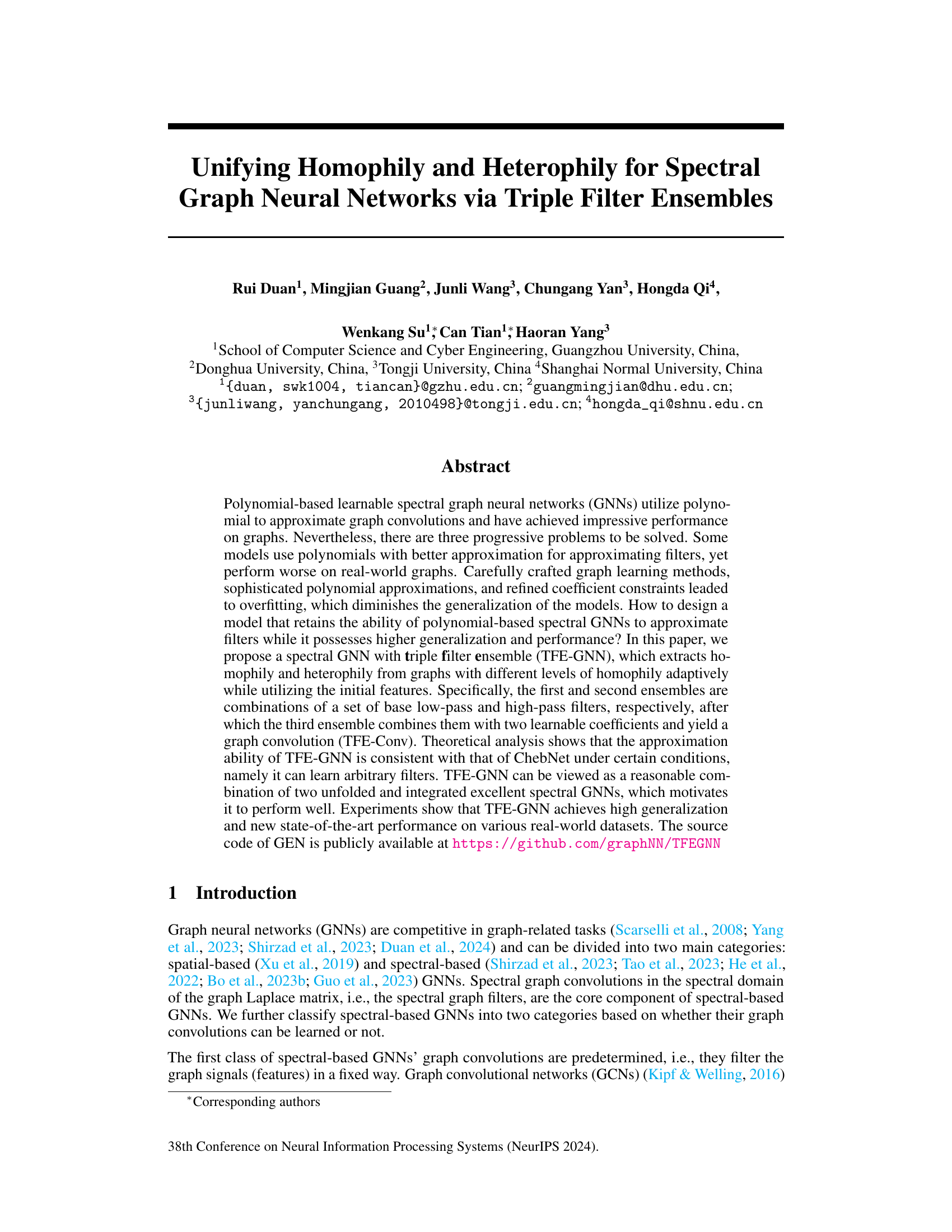
This figure illustrates the architecture of the Triple Filter Ensemble Graph Neural Network (TFE-GNN). It starts with a graph (G) as input. The graph’s initial features are then filtered by a triple filter ensemble mechanism (TFE). This mechanism first constructs two ensembles, one for low-pass filters (extracting homophily) and one for high-pass filters (extracting heterophily). These two ensembles are combined in a third ensemble with learnable coefficients (v1, v2), producing a graph convolution. This filtered signal is then passed through a fully connected neural network (NN) and a softmax layer to generate the final prediction.

This table presents the statistics of eleven real-world datasets used in the paper for evaluating the performance of the proposed TFE-GNN model. For each dataset, it shows the number of nodes, edges, features, classes, and the edge homophily ratio (ehr). The ehr metric indicates the level of homophily (similarity of neighboring nodes) in the graph, ranging from 0.06 (strong heterophily) to 0.93 (strong homophily).
In-depth insights#
Triple Filter Ensemble#
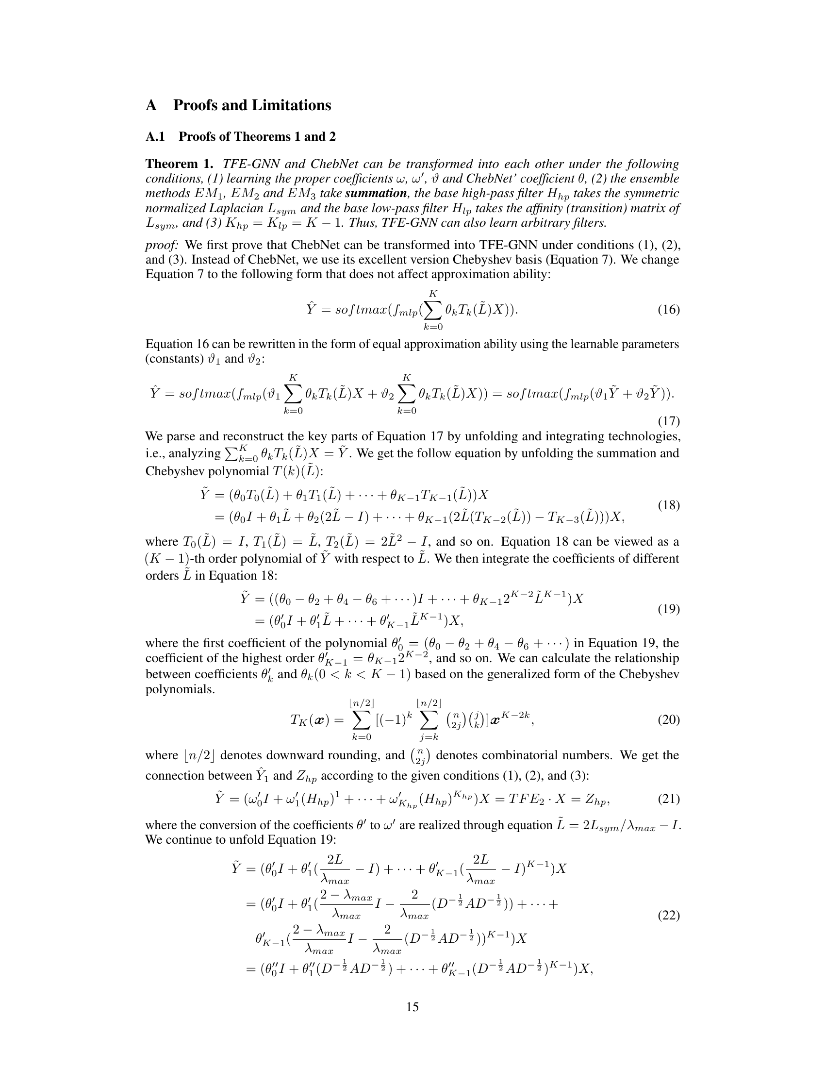
The Triple Filter Ensemble is a core concept in this research paper, aiming to enhance spectral graph neural networks (GNNs). It ingeniously combines three distinct filter ensembles: low-pass filters adept at capturing homophily (similarity among neighbors), high-pass filters for heterophily (dissimilarity), and a final ensemble that adaptively weighs the low-pass and high-pass results using learnable coefficients. This adaptive weighting is crucial, enabling TFE-GNNs to handle graphs with varying levels of homophily and heterophily effectively, a significant advance over previous GNN architectures that often struggle in such diverse scenarios. The use of ensembles promotes robustness and generalizability, mitigating overfitting and improving overall performance on real-world datasets. This approach is theoretically well-founded, showing consistency with established methods under certain conditions, making it a principled and promising improvement in spectral GNN design.
Adaptive Homophily#
Adaptive homophily in graph neural networks (GNNs) addresses the challenge of handling graphs with varying degrees of homophily (the tendency of similar nodes to connect). Traditional GNNs often struggle with heterophilic graphs (where dissimilar nodes connect frequently), as their inductive biases favor homophily. Adaptive homophily methods aim to dynamically adjust the model’s behavior based on the local homophily level within the graph. This might involve learning different aggregation functions or filter parameters for homophilic and heterophilic regions, or using attention mechanisms to weight the contributions of neighbors based on their similarity to the central node. The key benefit is improved generalizability to diverse real-world graphs, which often exhibit mixed homophily patterns. A successful adaptive homophily approach should not only improve performance on heterophilic graphs but also maintain competitiveness on homophilic graphs. Careful design is needed to avoid overfitting to specific homophily levels, and robust evaluation across a spectrum of graph types is crucial to demonstrate effectiveness.
Spectral GNN#
Spectral Graph Neural Networks (GNNs) operate in the frequency domain, leveraging the spectral decomposition of the graph Laplacian matrix. This approach offers several advantages: powerful expressiveness in capturing graph structure through spectral filters, theoretical grounding in signal processing, and the ability to learn filters adaptively for various graph properties. However, challenges exist such as the computational cost of spectral decomposition for large graphs, the difficulty in directly interpreting the learned filters in the spectral domain, and the sensitivity to noise in the graph data. Polynomial-based methods are widely used to approximate spectral convolutions, but carefully crafted graph learning or sophisticated polynomial approximations can lead to overfitting. Recent research focuses on addressing these challenges through techniques like filter ensemble methods, improved polynomial approximations, and more efficient spectral filtering operations for increased efficiency and generalization. The key is finding a balance between the expressive power of spectral GNNs and the practical constraints of scalability and interpretability.
Generalization#
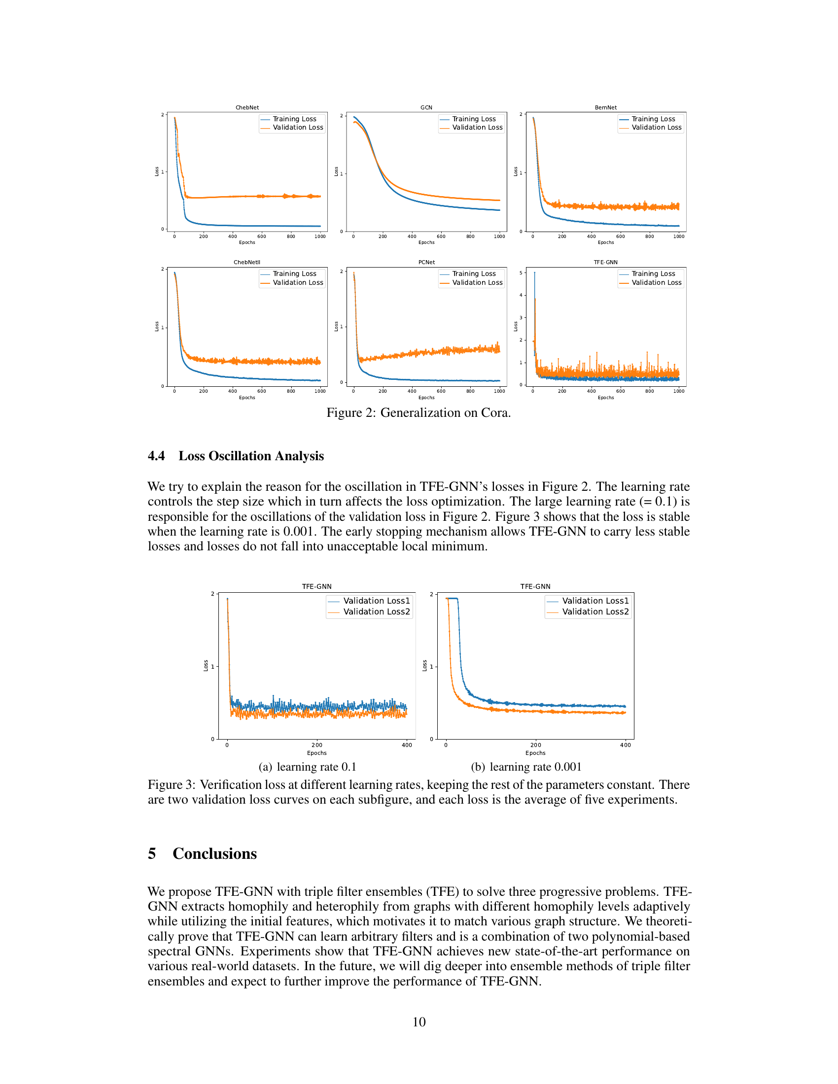
Generalization in machine learning models, especially deep learning models, refers to a model’s ability to perform well on unseen data that was not part of its training set. The paper investigates the generalization capabilities of a novel graph neural network (GNN) architecture. Overfitting is a major challenge to generalization, where a model performs exceptionally well on the training data but poorly on new data. The authors address this by proposing a novel triple filter ensemble mechanism, which combines homophily and heterophily graph filters adaptively. This approach reduces overfitting by creating a more robust and generalized model that isn’t overly sensitive to the training data’s specific characteristics. The empirical results of the experiments demonstrate that TFE-GNN achieves high generalization performance across numerous real-world datasets, showcasing its effectiveness. Theoretical analysis further supports these findings, establishing a connection between the model and well-established spectral GNNs. The analysis demonstrates that under certain conditions, the proposed model can learn arbitrary filters, thus enhancing its capacity to generalize. Careful attention is paid to various homophily levels across datasets, highlighting the model’s adaptability. This leads to state-of-the-art performance.
Future Work#
Future research directions stemming from this work could explore several promising avenues. Extending TFE-GNN to handle dynamic graphs would significantly broaden its applicability, enabling it to tackle real-world scenarios where graph structures evolve over time. Investigating more sophisticated ensemble methods beyond the triple filter ensemble, perhaps incorporating techniques from boosting or stacking, could potentially further improve performance and robustness. A deeper theoretical analysis of TFE-GNN’s approximation capabilities, particularly under more general conditions, would solidify its mathematical foundations. Furthermore, exploring applications beyond node classification, such as graph classification, link prediction, or graph generation, would demonstrate its versatility. Finally, a comprehensive empirical evaluation on a wider range of datasets, including those with diverse characteristics and homophily levels, would strengthen the findings and enhance its generalizability.
More visual insights#
More on figures
This figure illustrates the architecture of the Triple Filter Ensemble Graph Neural Network (TFE-GNN). It shows how three ensembles of filters (low-pass, high-pass, and a combined ensemble) are used to extract homophily and heterophily from graph signals. The filtered signals are then passed through a fully connected neural network and a softmax layer for prediction. The diagram visually represents the process of combining low and high-pass filters to adaptively extract features from graphs, representing both homophilic and heterophilic relationships.
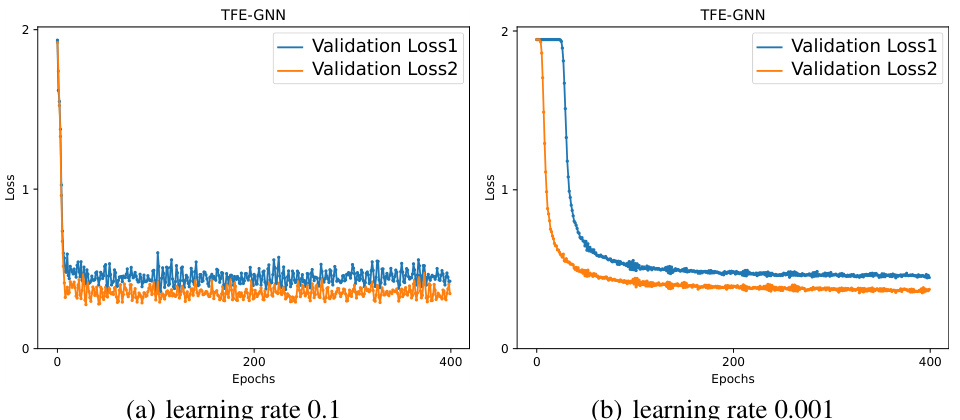
This figure shows the effect of the learning rate on the stability of the training process. Two different learning rates were tested: 0.1 (left) and 0.001 (right). The plots show the validation loss for both learning rates. The plot on the left, with a learning rate of 0.1, shows a less stable training process with more oscillations in the validation loss. The plot on the right, with a learning rate of 0.001, shows a more stable training process with fewer oscillations, indicating that the lower learning rate leads to better convergence.

This figure illustrates the architecture of the Triple Filter Ensemble Graph Neural Network (TFE-GNN). It shows how low-pass and high-pass filters are combined through ensembles to create a graph convolution (TFE-Conv), which is then fed into a fully connected neural network for prediction. The figure highlights the adaptive extraction of homophily and heterophily from graphs with varying homophily levels.

This figure illustrates the architecture of the Triple Filter Ensemble Graph Neural Network (TFE-GNN). It shows how the network combines low-pass and high-pass filters to extract both homophily and heterophily information from the graph, ultimately leading to a more robust and accurate representation. The process begins with the input features of the graph, which are then passed through separate low-pass and high-pass filter ensembles. These ensembles are combined using learnable coefficients, producing a final graph convolution, which is then fed into a fully connected neural network for prediction. The TFE-GNN is designed to adaptively extract homophily and heterophily information from graphs with different levels of homophily, and it utilizes the initial features to improve accuracy.

This figure illustrates the architecture of the Triple Filter Ensemble Graph Neural Network (TFE-GNN). It shows how the base low-pass and high-pass filters are combined through ensemble methods (EM1, EM2) to form the first and second ensembles. These ensembles are further combined using two learnable coefficients (v1, v2) and another ensemble method (EM3) to generate the final graph convolution (TFE-Conv). The output of TFE-Conv is then fed into a fully connected neural network (NN), which produces the final prediction after a softmax layer. The figure clearly demonstrates the adaptive extraction of homophily and heterophily from graphs using this novel triple filter ensemble mechanism.

This figure illustrates the architecture of the Triple Filter Ensemble Graph Neural Network (TFE-GNN). It shows how the model combines low-pass and high-pass filters to adaptively extract homophily and heterophily from graphs. The process starts with the input features, then uses three filter ensembles: the first ensemble combines low-pass filters, the second combines high-pass filters, and the third combines the outputs of the first two ensembles with learnable coefficients. Finally, a fully connected neural network and a softmax layer provide the output prediction.
More on tables

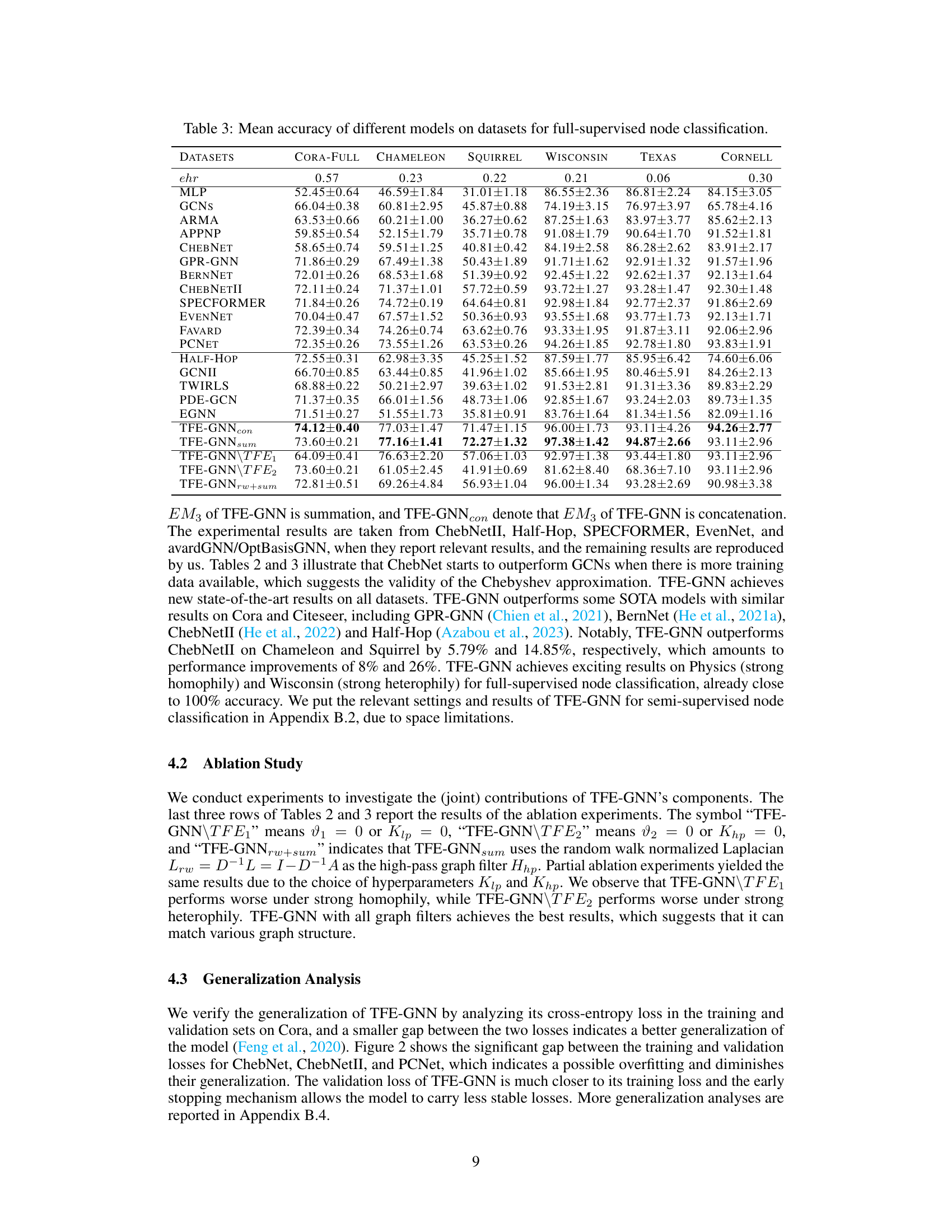
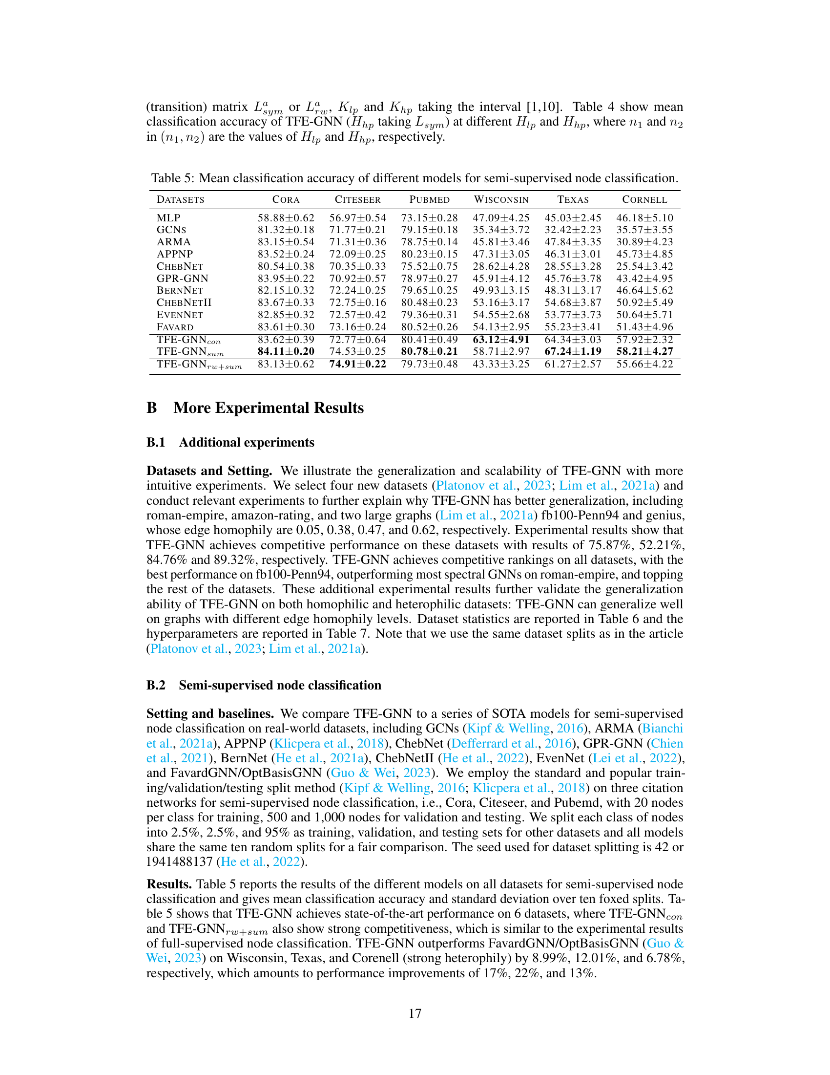
This table presents the mean accuracy and standard deviation of various graph neural network (GNN) models on eleven real-world datasets for the task of full-supervised node classification. The results are averaged across ten random dataset splits. The table allows for comparison of the performance of TFE-GNN against existing state-of-the-art GNN models across datasets with varying levels of homophily (ehr).
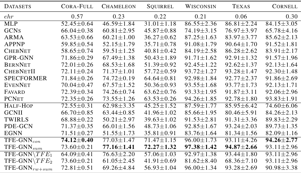
This table presents the mean accuracy of various graph neural network (GNN) models on eleven datasets for a full-supervised node classification task. The results are averaged over ten random splits, and error bars (standard deviations) are included to indicate variability. The table allows for a comparison of the performance of TFE-GNN against other state-of-the-art (SOTA) GNN models. Datasets are grouped by their edge homophily ratio (ehr), offering insight into the models’ performance across different homophily levels.

This table shows the mean classification accuracy of different models with varying low-pass (Hip) and high-pass (Hhp) filter settings. The results are presented for two datasets: Citeseer and Wisconsin. Different combinations of Hip and Hhp values are tested, allowing for the analysis of how these parameters affect model performance on datasets with varying levels of homophily.

This table presents the mean accuracy achieved by various graph neural network (GNN) models on eleven real-world datasets for the task of full-supervised node classification. The results are reported as mean accuracy ± standard deviation, calculated over ten random dataset splits. The table allows a comparison of the performance of TFE-GNN against state-of-the-art (SOTA) methods, highlighting TFE-GNN’s superior performance on most datasets.

This table presents the key statistics for four additional datasets used in the experiments beyond the initial eleven. These statistics include the number of nodes, edges, features (node attributes), classes (number of categories for node labels), and the edge homophily ratio (ehr). The ehr metric quantifies the level of homophily (similarity of connected nodes) within each graph, ranging from very low (0.05) to moderately high (0.62).

This table shows the hyperparameters used for TFE-GNN on four additional datasets: roman-empire, amazon-rating, fb100-Penn94, and genius. The hyperparameters include the optimizer, the order of the low-pass and high-pass graph filters (Klp and Khp), dropout rates for input and intermediate features, learning rates and weight decay for various learnable coefficients, and learning rates and weight decay for the MLP. These settings were used for the experiments evaluating the model’s performance.

This table presents the training time (in seconds) for different graph neural networks (GNNs) on the Cora dataset. The time is measured for various values of K, representing the order of the Chebyshev polynomials used in the GNNs. The table compares the training time of ChebNet, BernNet, ChebNetII, and three variants of TFE-GNN (with different configurations of Klp and Khp). This allows for an analysis of the impact of model complexity and hyperparameter settings on training efficiency.

This table presents the mean accuracy and standard deviation of different graph neural network models on eleven benchmark datasets for the task of full-supervised node classification. The results are averaged over ten random splits. The datasets vary in size, number of features, and importantly, their level of homophily (as measured by the edge homophily ratio, ’ehr’). This allows for a comparison of the models’ performance across different graph characteristics.
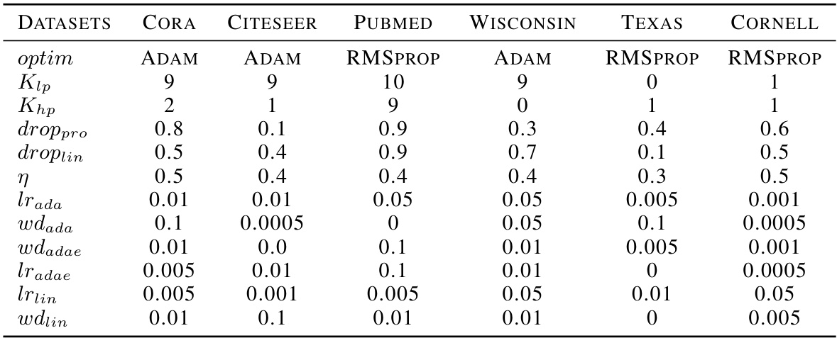
This table shows the hyperparameter settings used for the TFE-GNN model in the semi-supervised node classification experiments. It lists the optimizer used (optim), the orders of low-pass (Klp) and high-pass (Khp) filters, dropout rates for input and intermediate features (droppro and droplin), learning rates for different sets of coefficients (η, lrada, lradae, lrlin), and weight decay values (wdada, wdadae, wdlin). The values vary depending on the dataset used.
Full paper#
