↗ OpenReview ↗ NeurIPS Homepage ↗ Chat
TL;DR#
Many industrial applications demand accurate forecasts across various time horizons; however, existing time-series models often require separate training and deployment for each horizon, limiting flexibility and efficiency. Pre-trained universal models offer some improvement but lack in-depth investigation into varied-horizon forecasting challenges.
The paper introduces ElasTST, an Elastic Time-Series Transformer, designed to address this limitation. ElasTST uses a non-autoregressive architecture with placeholders and structured attention masks to ensure horizon-invariant outputs. A tunable version of rotary position embedding enhances adaptability to various horizons, while a multi-scale patch design effectively integrates fine-grained and coarse-grained information. Experiments demonstrate ElasTST’s superior performance compared to existing models, showing its effectiveness and robustness across different horizons and datasets. ElasTST’s open-source availability further enhances its impact on the field.
Key Takeaways#
Why does it matter?#
This paper is crucial because it addresses a critical gap in time-series forecasting, where current methods struggle with varied-horizon forecasting. The proposed ElasTST model offers a robust and efficient solution, paving the way for improved applications in diverse fields and enabling new research into efficient, universal time-series models.
Visual Insights#

This figure provides a detailed overview of the ElasTST architecture, highlighting its key components: structured attention masks for handling varied forecasting horizons, tunable rotary position embedding (ROPE) for adapting to time series periodicities, multi-scale patch assembly for integrating fine-grained and coarse-grained information, and a horizon reweighting scheme for efficient training across multiple horizons. Each component is illustrated with a subfigure, explaining its role in achieving robust and consistent forecasting performance.
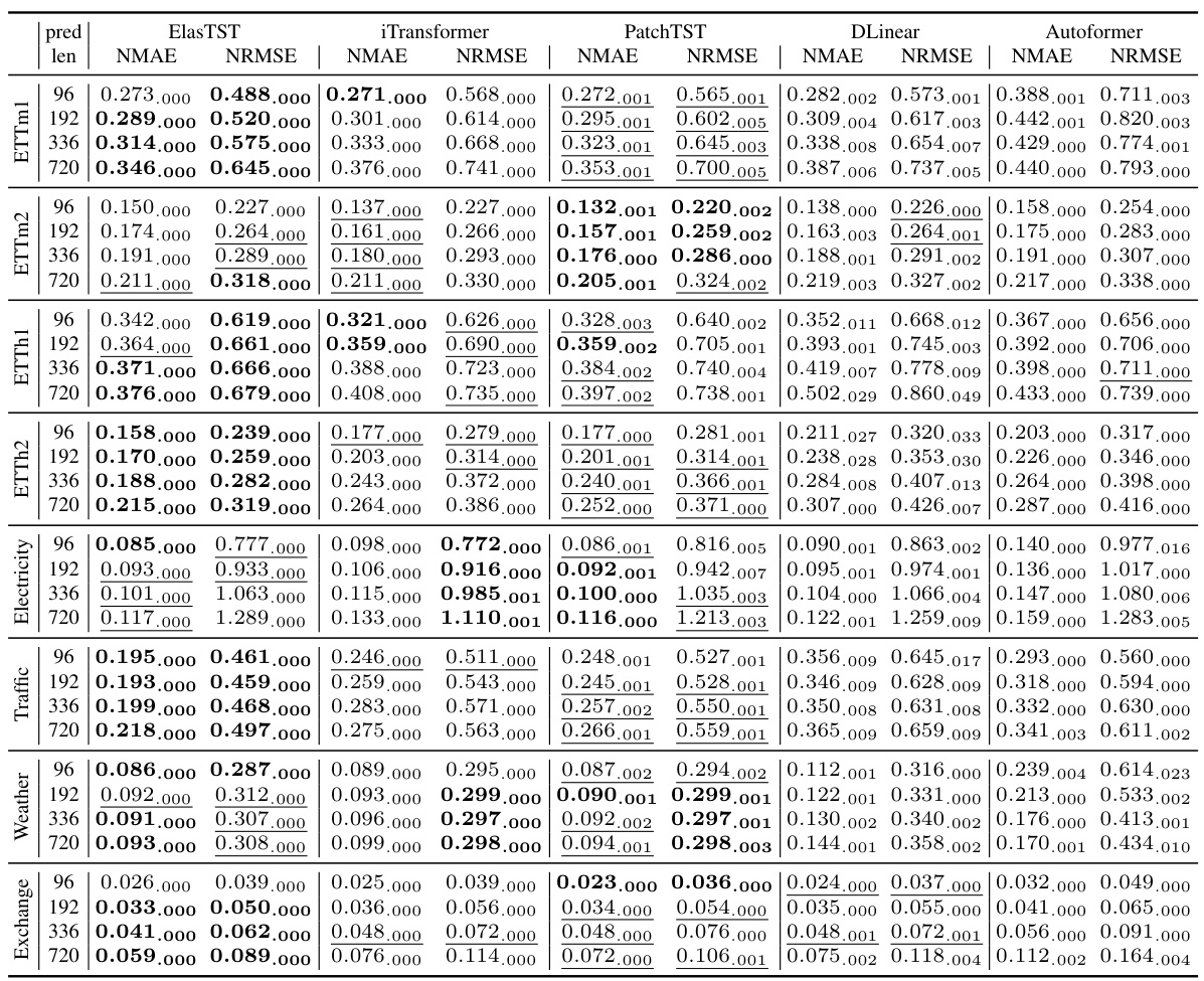
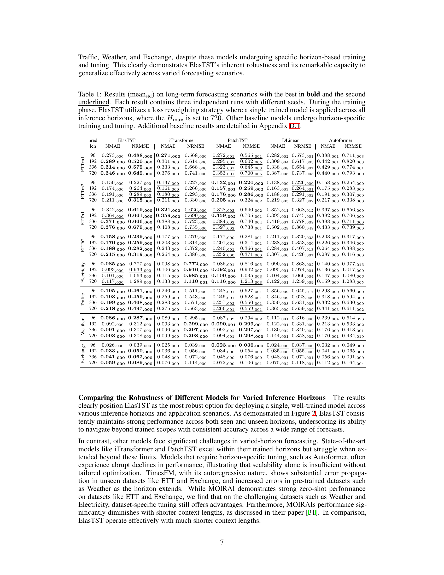
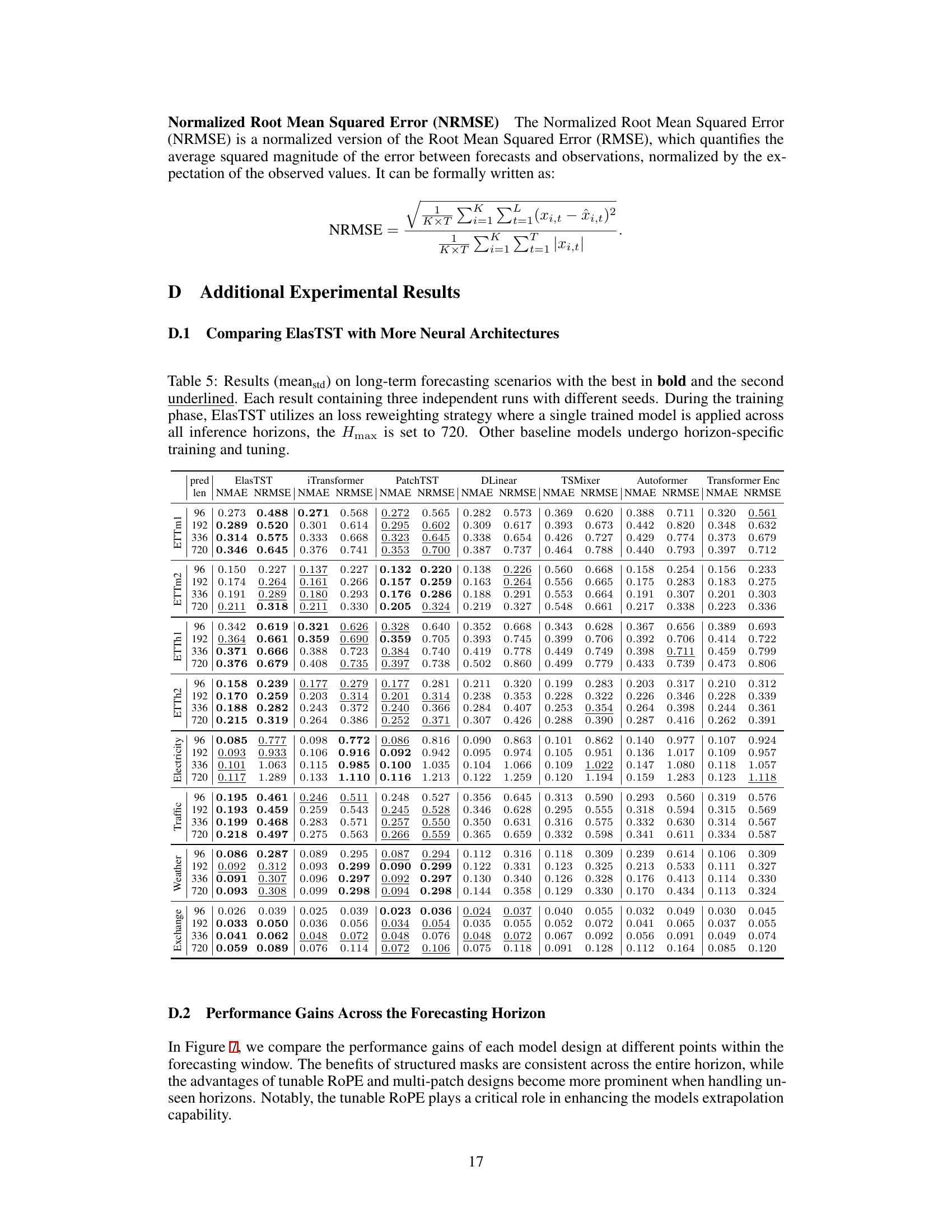
This table presents the main results of the paper, comparing the performance of ElasTST with other state-of-the-art time series forecasting models across various datasets and forecasting horizons. ElasTST uses a reweighting scheme to train a single model effective for all forecast horizons. Other models are trained and tuned for specific horizons. Results are reported as mean ± standard deviation, across three independent runs.
In-depth insights#
Elastic Forecasting#
Elastic forecasting, a concept not explicitly defined in the provided text, can be interpreted as a flexible and adaptive approach to time series prediction. It addresses the challenge of traditional forecasting models that struggle with varied horizons or changing data characteristics. A truly elastic model would dynamically adjust its architecture and parameters, automatically handling unseen data patterns or forecast horizons without requiring retraining or hyperparameter tuning. This necessitates a non-autoregressive architecture, possibly using placeholders or attention mechanisms to handle variable-length outputs and inputs. Multi-scale features would also likely be incorporated to deal with short and long-term dynamics simultaneously. Transfer learning and pre-training could further enhance adaptability, allowing the model to generalize effectively to new datasets with minimal fine-tuning. The development of such models would be a significant step forward in creating more robust and efficient time series forecasting systems that readily handle diverse and dynamic real-world scenarios.
Tunable RoPE#
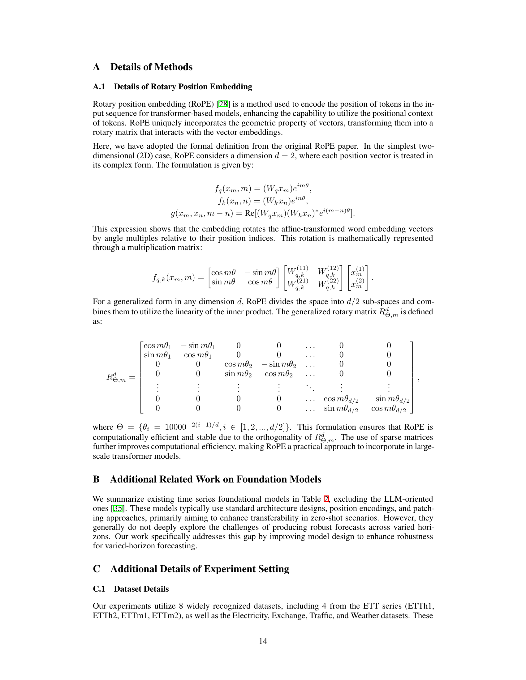
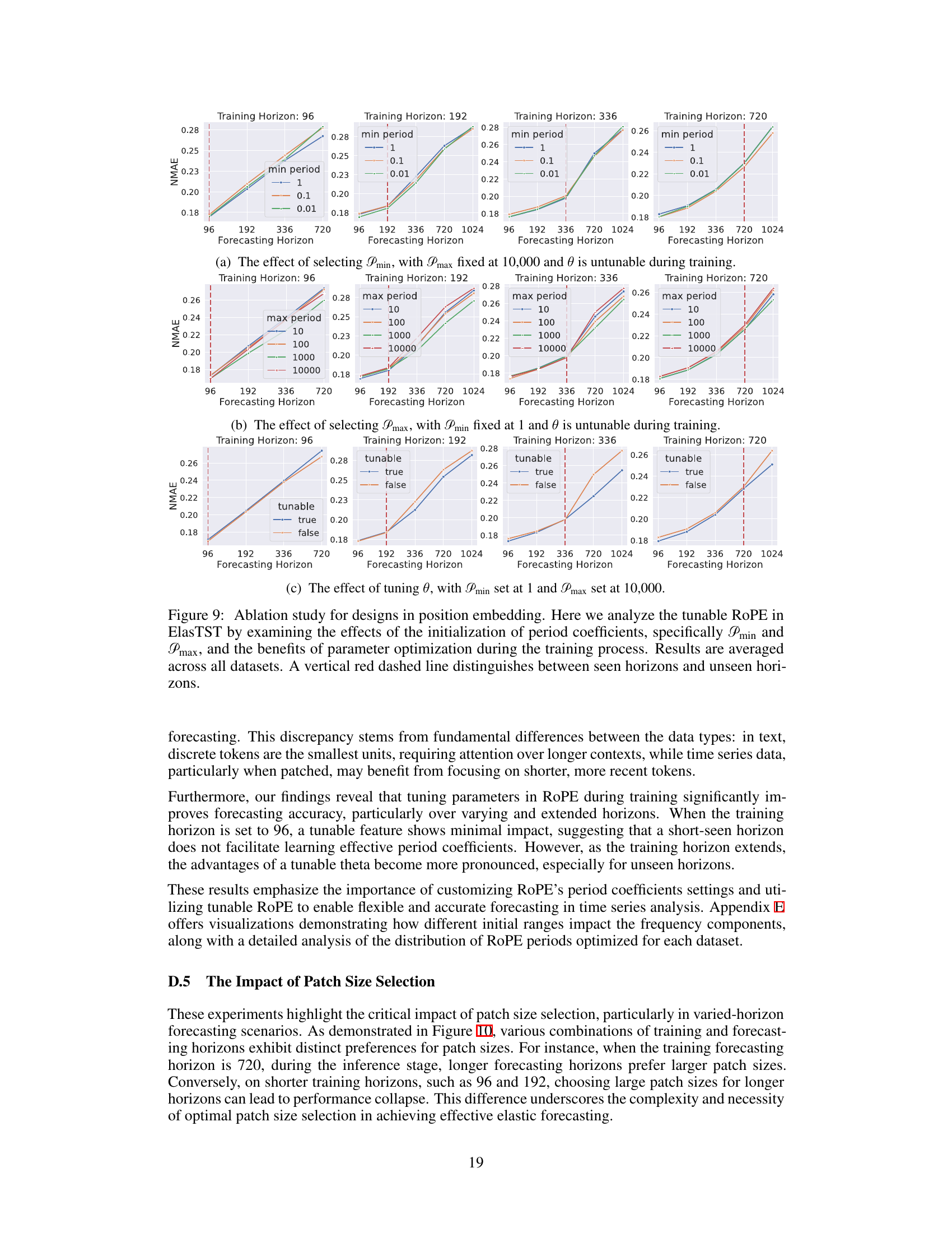
The proposed “Tunable RoPE” method presents a notable enhancement to standard Rotary Position Embedding (RoPE) for time-series forecasting. Traditional RoPE, while effective in handling variable-length sequences in NLP, doesn’t optimally adapt to the inherent periodic patterns frequently found in time-series data. The key innovation is the introduction of tunable period coefficients, allowing the model to learn and adapt to these dataset-specific periodicities, rather than relying on fixed, pre-defined values. This dynamic adjustment allows for a more nuanced and accurate representation of temporal relationships, particularly crucial for longer forecasting horizons where traditional methods struggle. The approach leverages an exponential distribution of period coefficients, mirroring the original RoPE setup but offering greater flexibility and alignment with time-series characteristics. This demonstrably improves forecasting accuracy and extrapolation capabilities, particularly on unseen horizons, as evidenced by the experimental results.
Multi-Scale Patches#
Employing multi-scale patches in time-series forecasting offers a powerful mechanism to capture both fine-grained and coarse-grained information. Fine-grained patches excel at modeling short-term, high-frequency fluctuations, while coarse-grained patches better capture long-term trends and low-frequency patterns. Combining these perspectives within a single model architecture allows for a more comprehensive and nuanced understanding of the time series dynamics. This approach is particularly beneficial for varied-horizon forecasting, as it enables the model to adapt to different temporal resolutions depending on the forecasting horizon. A key challenge is determining the optimal patch sizes and how best to integrate the information from different scales. The paper’s innovative multi-scale patch assembly method tackles this challenge by merging fine and coarse-grained information, showing the effectiveness of the combined information in producing more robust and accurate predictions across various forecasting horizons.
Horizon Reweighting#
The ‘Horizon Reweighting’ strategy, as described in the paper, is a clever method to address the challenge of training a time-series forecasting model on multiple horizons without the need for extensive and computationally expensive resampling. Instead of generating numerous training instances by randomly selecting various forecasting horizons, it employs a reweighting scheme during the training process, effectively simulating the effects of such resampling using a single fixed horizon. This approach is especially advantageous because it significantly reduces training time and computational cost. The core idea is to approximate the expected loss across multiple horizons by weighting the loss function based on the inverse of the horizon length. This weighted loss is then utilized during training, creating a robust model adaptable to varied-horizon forecasting. The strategy appears efficient and effective in approximating the benefit of multiple horizon training, which is a significant improvement over traditional methods that require separate training and model maintenance for each horizon. This allows a single model to handle a wide range of forecast horizons effectively, making it a practical solution for real-world applications.
Future Work#
The “Future Work” section of this research paper offers several promising avenues. Extending ElasTST’s capabilities through pre-training is crucial, potentially leveraging a massive dataset to enhance its generalizability and zero-shot performance. Investigating different architectural modifications, such as exploring alternative attention mechanisms or incorporating other advanced techniques, could further optimize performance and robustness. Addressing the current limitations by testing the model on a more diverse range of datasets, including those with varying complexities and characteristics, would validate its practical applicability across different industrial domains. Finally, a deeper exploration of hyperparameter optimization techniques specific to ElasTST would improve the model’s efficiency and training process, potentially reducing computational costs and improving performance further. A comparative analysis of the relative efficiency of different implementations is also warranted to ensure optimization for diverse hardware environments.
More visual insights#
More on figures

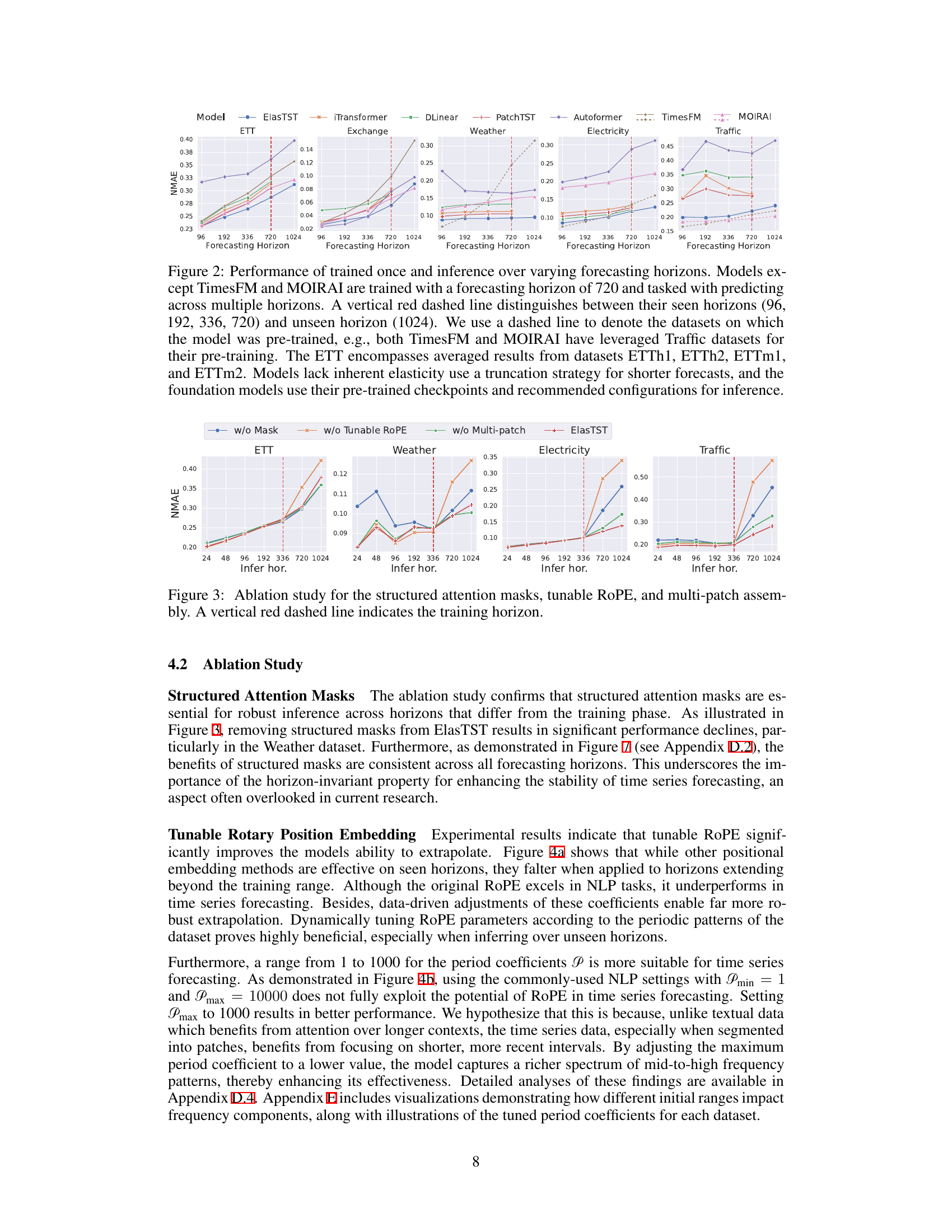
This figure compares the performance of various time series forecasting models across different forecasting horizons. Models were trained on a horizon of 720, then tested on shorter and longer horizons to assess their robustness and ability to generalize. The figure shows that ElasTST maintains consistent accuracy across all horizons, outperforming other models which struggle when predicting beyond their training horizon.

This figure compares the performance of ElasTST and other models across various forecasting horizons, including unseen horizons. It demonstrates ElasTST’s robustness and ability to generalize well compared to models trained for specific horizons.
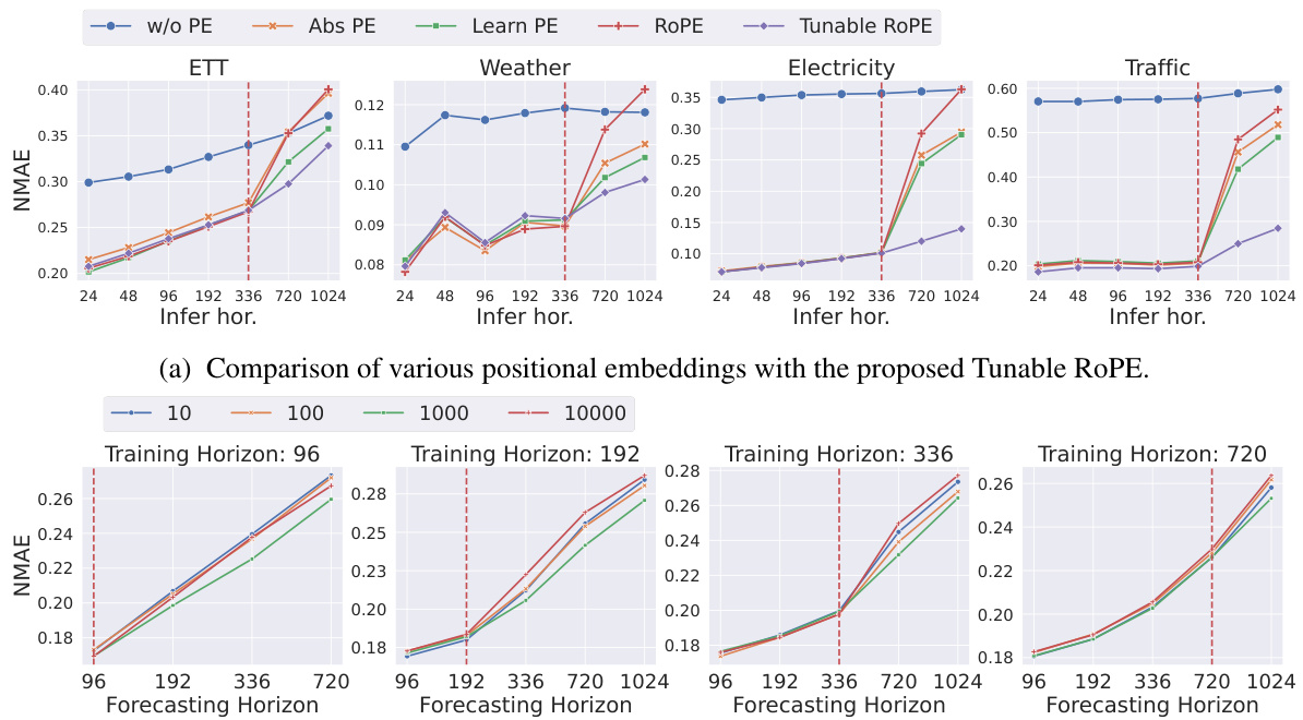
This figure compares the performance of ElasTST and other time series forecasting models across various forecasting horizons, both seen and unseen during training. It highlights ElasTST’s ability to maintain strong performance across different horizons without needing per-horizon training.

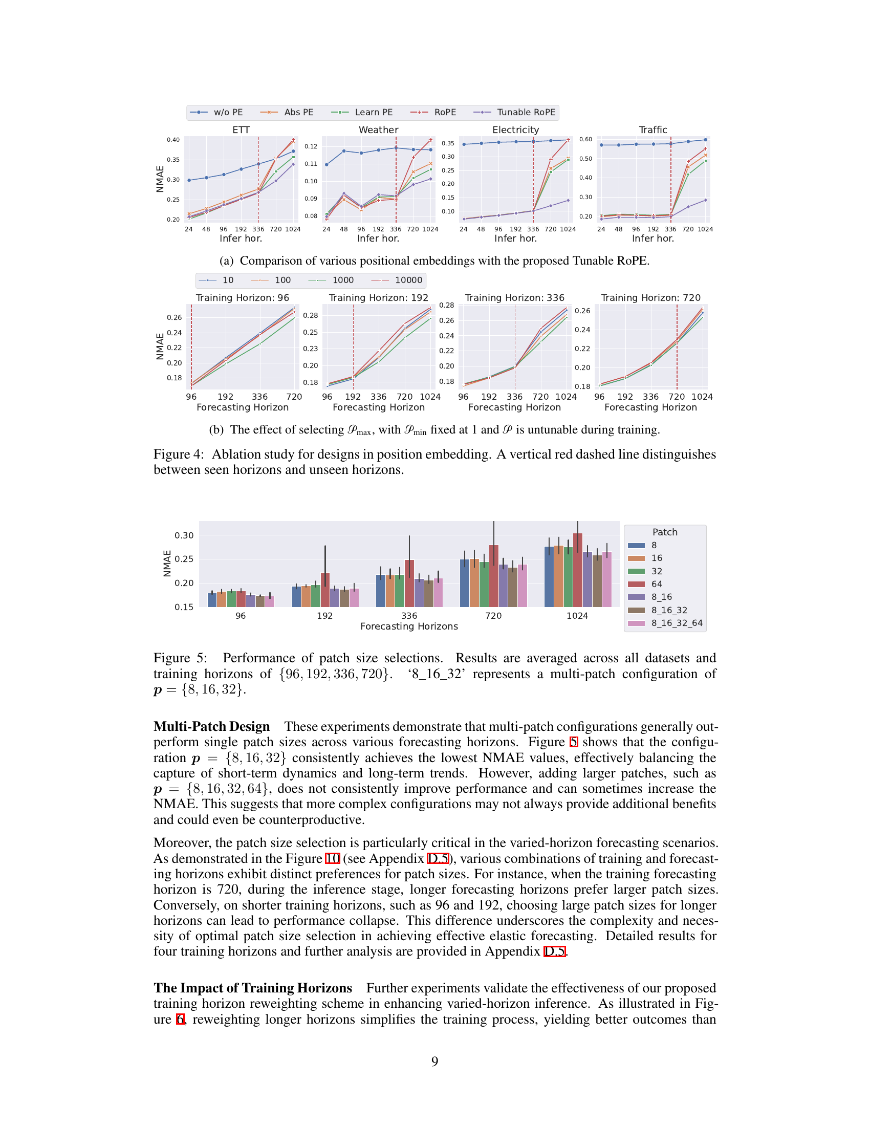
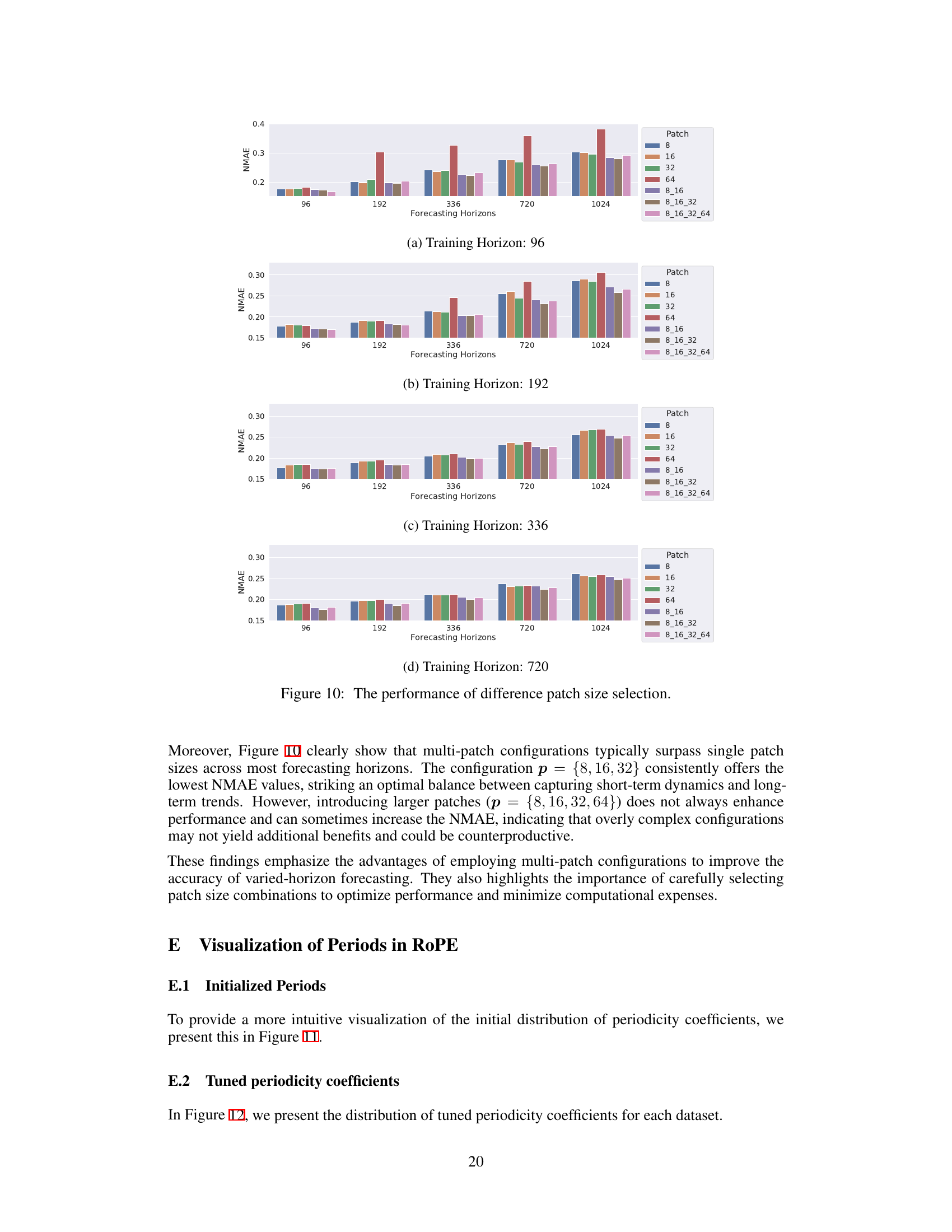
The figure shows the effect of different patch sizes on forecasting performance across various forecasting horizons. It compares single patch sizes (8, 16, 32, 64) with multi-patch configurations (combining these sizes). The results suggest that a multi-patch approach (e.g., 8, 16, and 32) generally outperforms single patch sizes, achieving a better balance between capturing short-term dynamics and long-term trends. However, adding very large patches does not always improve performance and might even be counterproductive.

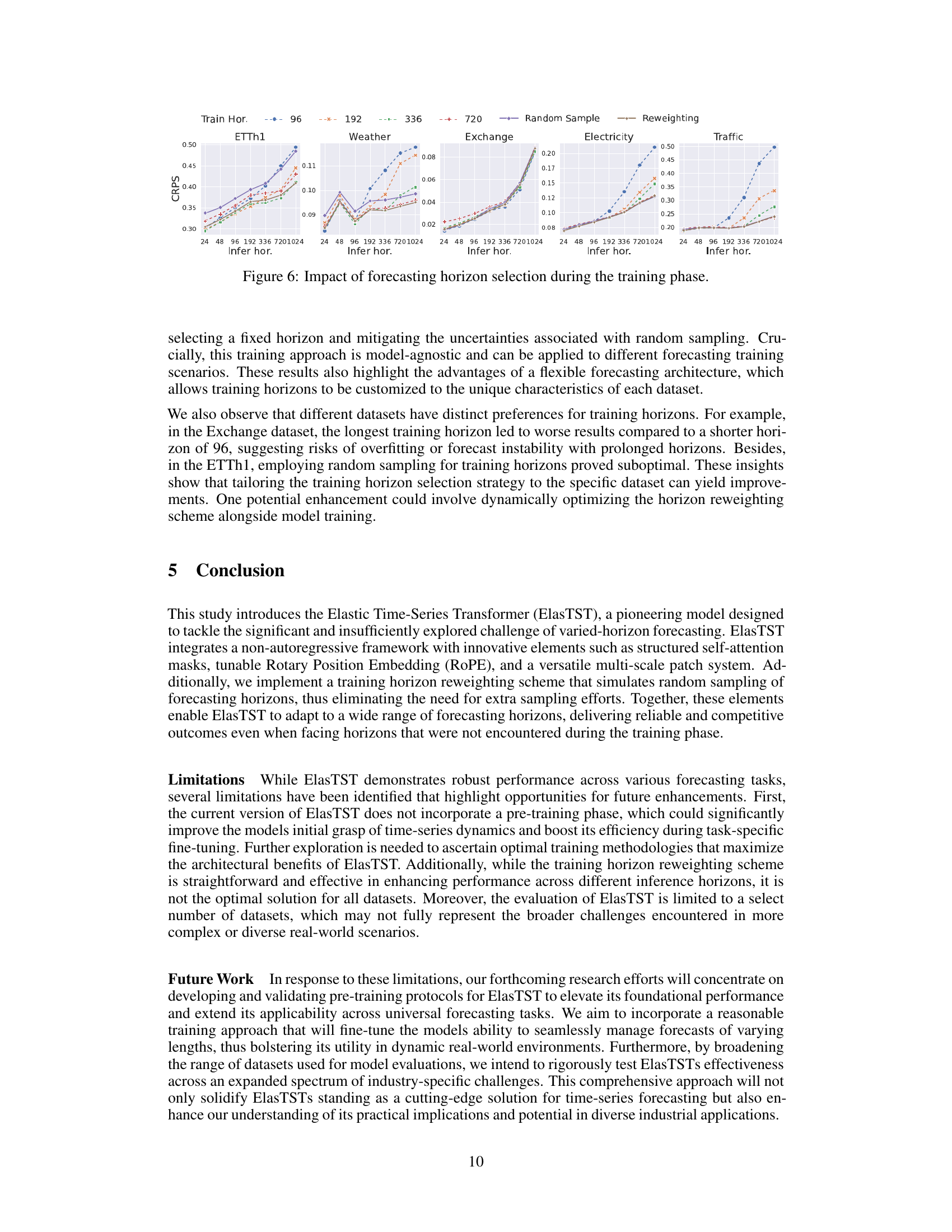
This figure visualizes the impact of different training horizon lengths on forecasting performance across various inference horizons. It compares the results of training with fixed horizons (96, 192, 336, 720) against the results of training with randomly sampled horizons and the proposed reweighting scheme. The results are displayed using CRPS (Continuous Ranked Probability Score) as the evaluation metric for five different datasets. The figure aims to demonstrate the effectiveness of the proposed reweighting approach in simulating varied-horizon training using a single fixed training horizon, thus reducing computational costs and enhancing the model’s generalization ability across various forecast lengths.

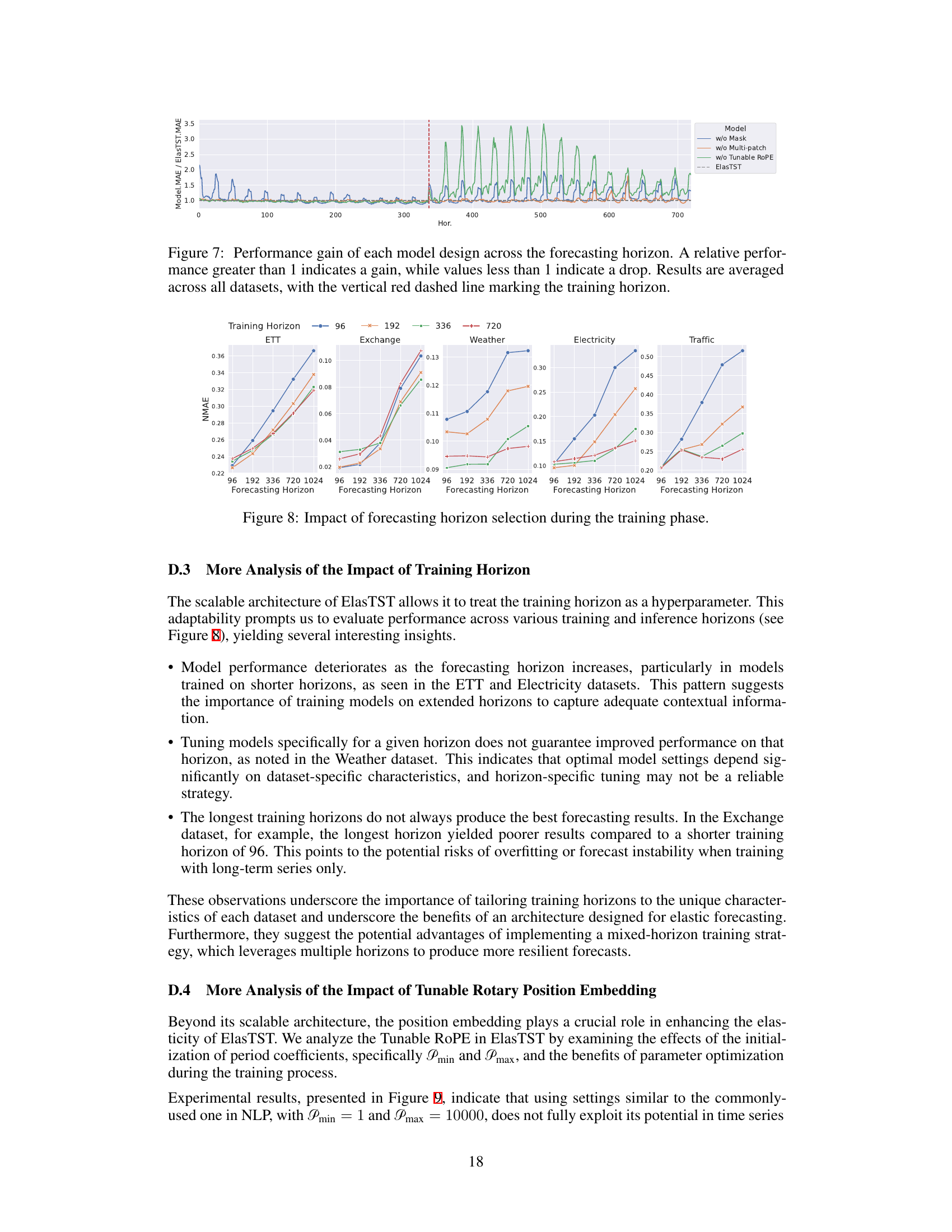
This figure shows the relative performance improvement of ElasTST compared to its variants without the structured attention mask, multi-patch assembly, or tunable RoPE. The x-axis represents the forecasting horizon, and the y-axis shows the ratio of the MAE for each variant to the MAE for the full ElasTST model. Values above 1 indicate that ElasTST outperforms the variant, while values below 1 indicate the opposite. The red dashed line marks the training horizon. This visualization helps to understand the contribution of each design element to the model’s performance across different forecasting horizons.

This figure compares the performance of ElasTST and other forecasting models across various forecasting horizons, both seen (during training) and unseen (during inference). It highlights ElasTST’s robustness in maintaining performance across different horizons while other models struggle, especially in extrapolating to unseen horizons.

This figure compares the performance of various time series forecasting models across different forecasting horizons. Models are trained on a single horizon (720) and then tested on a range of horizons. The figure shows that ElasTST maintains consistent accuracy across both seen and unseen horizons, while other models show degradation in performance for unseen horizons.
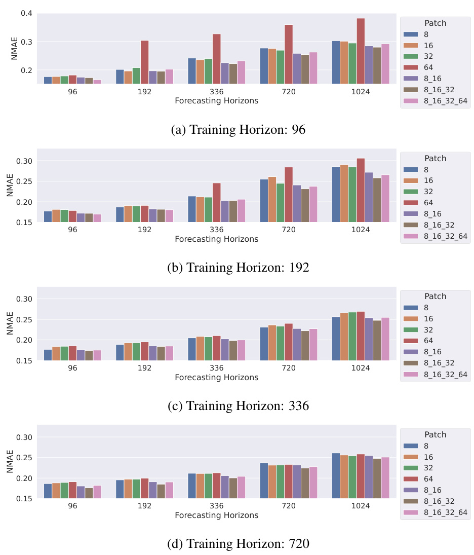
The figure shows the impact of different patch sizes on forecasting performance across various forecasting horizons and training horizons. It compares the performance of single patch configurations (using only one patch size: 8, 16, 32, or 64) to multi-patch configurations which combine multiple patch sizes (e.g., 8, 16, and 32). The results are presented as NMAE values across different forecasting horizons for each training horizon (96, 192, 336, and 720).
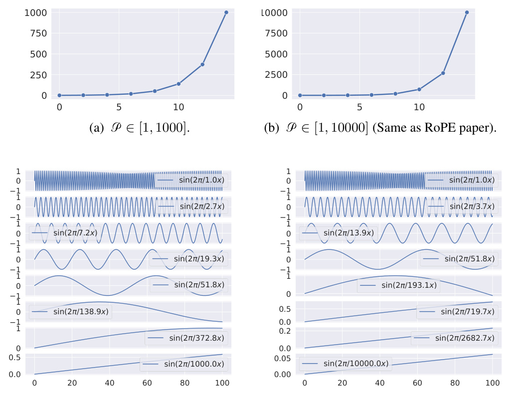
This figure compares the performance of ElasTST and several other models across various forecasting horizons, including an unseen horizon. It shows that ElasTST maintains strong performance even on unseen horizons, while others struggle, particularly those requiring per-horizon training or relying on autoregressive decoding. The figure highlights ElasTST’s robustness and generalization capabilities.

This figure provides a comprehensive overview of the ElasTST architecture, highlighting its key components: structured attention masks for handling varied forecasting horizons, tunable Rotary Position Embedding (ROPE) for adapting to time series periodicities, a multi-scale patch assembly for integrating both fine-grained and coarse-grained information, and a horizon reweighting scheme to simulate varied-horizon training.
More on tables

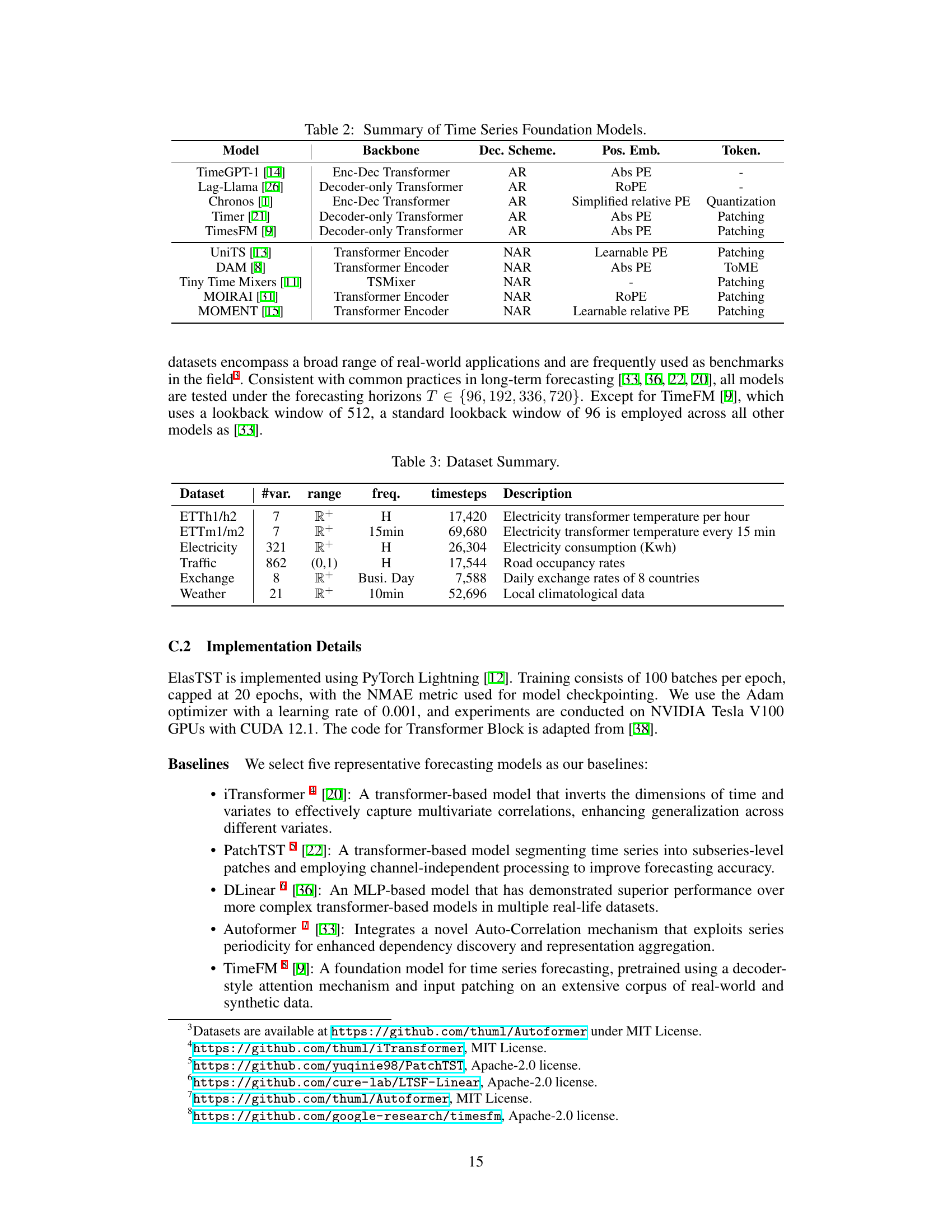
This table summarizes existing time series foundation models, excluding those based on LLMs. It compares the models based on their backbone architecture (Encoder-Decoder or Decoder-only Transformer), decoding scheme (Autoregressive or Non-Autoregressive), positional encoding methods, and tokenization techniques. The table provides context for understanding how ElasTST, the model presented in the paper, relates to and improves upon existing approaches.

This table presents the results of long-term forecasting experiments comparing ElasTST with other state-of-the-art models. ElasTST uses a reweighting scheme during training, allowing a single model to be used for all forecasting horizons, while other models are trained and tuned specifically for each horizon. The table shows the Normalized Mean Absolute Error (NMAE) and Normalized Root Mean Squared Error (NRMSE) for various prediction lengths (96, 192, 336, and 720) across multiple datasets.
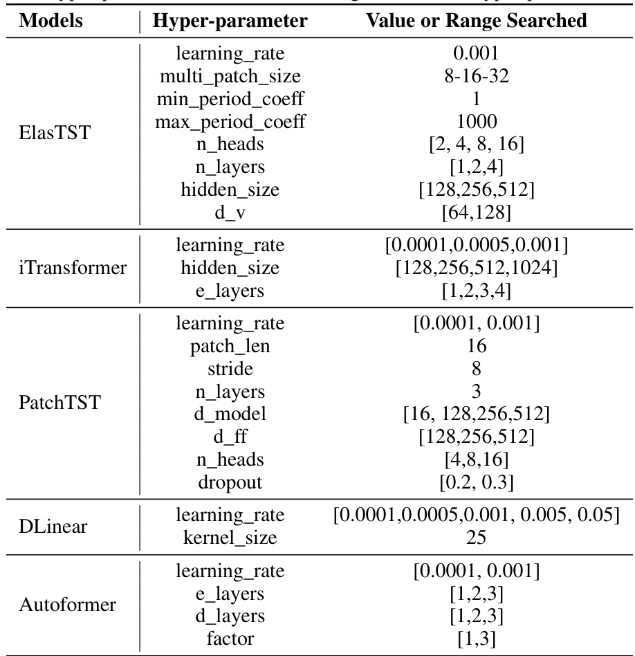
This table presents the results of long-term forecasting experiments comparing ElasTST with other state-of-the-art models. ElasTST uses a loss reweighting strategy during training to simulate varied forecasting horizons, whereas other models are trained and tuned specifically for each horizon. The table shows NMAE and NRMSE scores for various prediction lengths across multiple datasets.
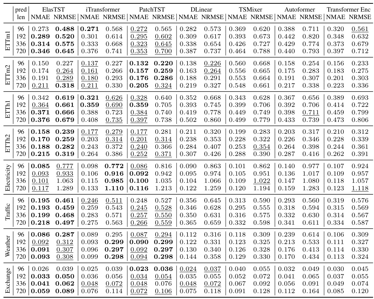
This table presents the results of long-term forecasting experiments comparing ElasTST with other state-of-the-art models. ElasTST uses a reweighting strategy during training, while other models are trained and tuned specifically for each horizon. The results show NMAE and NRMSE across various forecasting horizons (96, 192, 336, 720) and datasets (ETTm1, ETTm2, ETTh1, ETTh2, Electricity, Traffic, Weather, Exchange). Bold values indicate the best performance for each horizon/dataset combination.

This table presents the results of long-term forecasting experiments comparing ElasTST with other state-of-the-art models. It highlights ElasTST’s performance across various forecasting horizons (96, 192, 336, and 720) and datasets (ETTm1, ETTm2, ETTh1, ETTh2, Electricity, Traffic, Weather, and Exchange). The key takeaway is that ElasTST, trained with a reweighting scheme on a single horizon, achieves competitive or superior performance compared to models that were specifically trained and tuned for each horizon.

This table compares the maximum GPU memory usage and the number of parameters (NPARAMS) for ElasTST using three different position encoding methods: Absolute Position Embedding (Abs PE), Rotary Position Embedding (RoPE) without tunable parameters, and Rotary Position Embedding with tunable parameters (Tunable RoPE). It demonstrates the minimal memory overhead introduced by using RoPE.

This table shows the maximum GPU memory usage and the number of parameters (NPARAMS) for different patch size configurations in the ElasTST model. The configurations include using a single patch size (p=1, p=8, p=16, p=32) and multiple patch sizes (p={1,8,16,32}, p={8,16,32}). The results demonstrate the impact of patch size on memory consumption and model parameters.
Full paper#

