TL;DR#
Many machine learning applications, especially in imaging, deal with high-dimensional posterior distributions representing uncertainty in predictions. Visualizing these distributions is challenging, and existing methods often rely on sampling-based approaches, which can be computationally expensive and lack user-friendliness. This makes interpreting the uncertainty difficult and time-consuming for researchers.
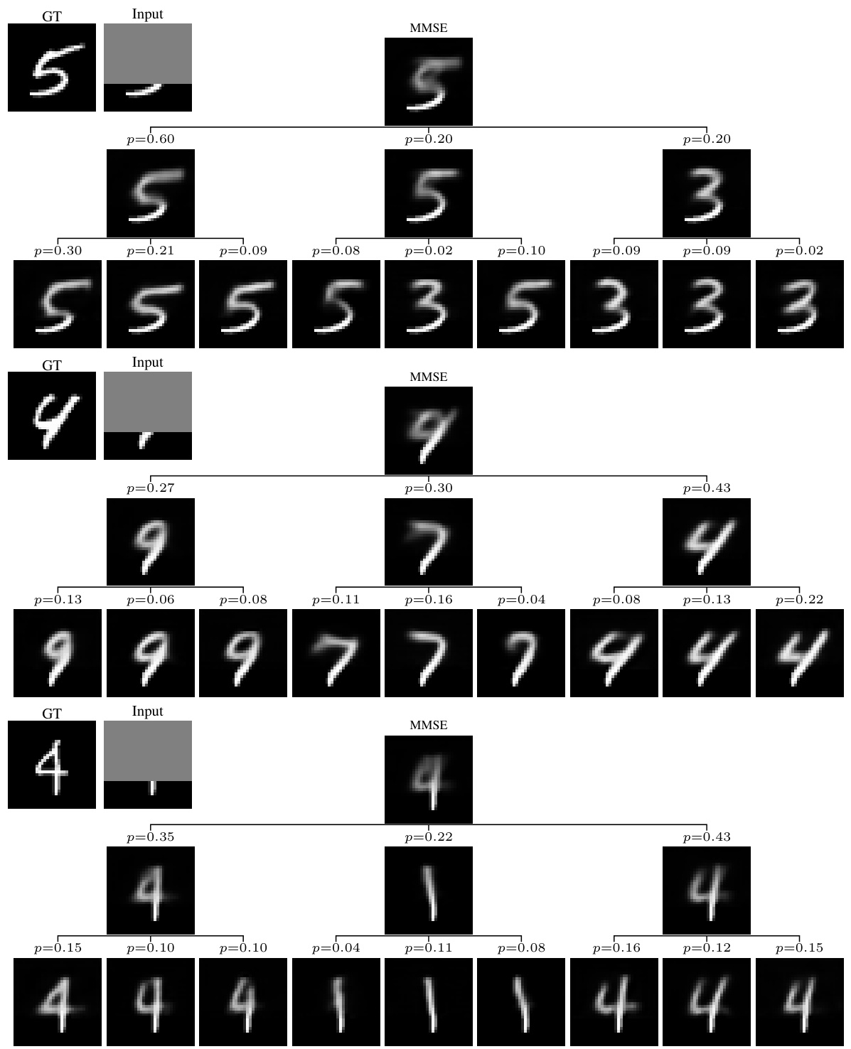
This research proposes a new method called ‘Posterior Trees’ to solve this. It uses a neural network to predict a tree-structured representation of the posterior, providing a hierarchical summary of uncertainty at various levels of granularity. The approach is significantly faster than sampling-based methods while maintaining comparable accuracy. The tree structure also makes the uncertainty information easier for users to understand and interact with.
Key Takeaways#
Why does it matter?#
This paper is significant because it presents a novel and efficient approach for visualizing high-dimensional posterior distributions, a common challenge in inverse problems. Its speed advantage over existing methods makes it practical for various applications, and the hierarchical tree structure offers a more intuitive and user-friendly way to explore uncertainties, advancing the reliability of machine learning models in areas where uncertainty quantification is crucial.
Visual Insights#

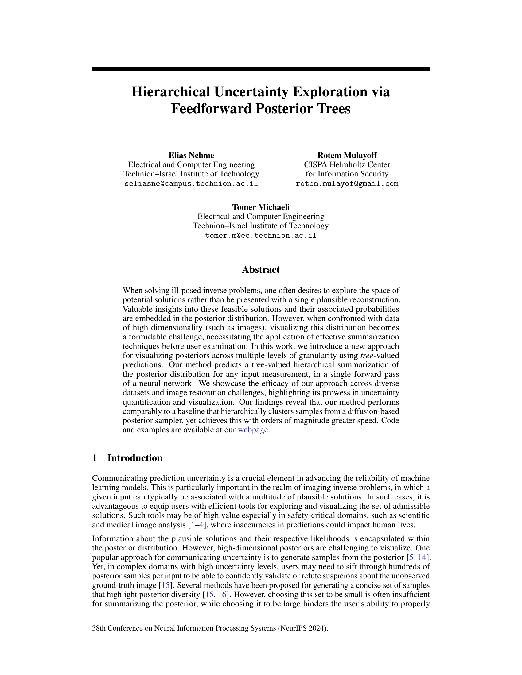
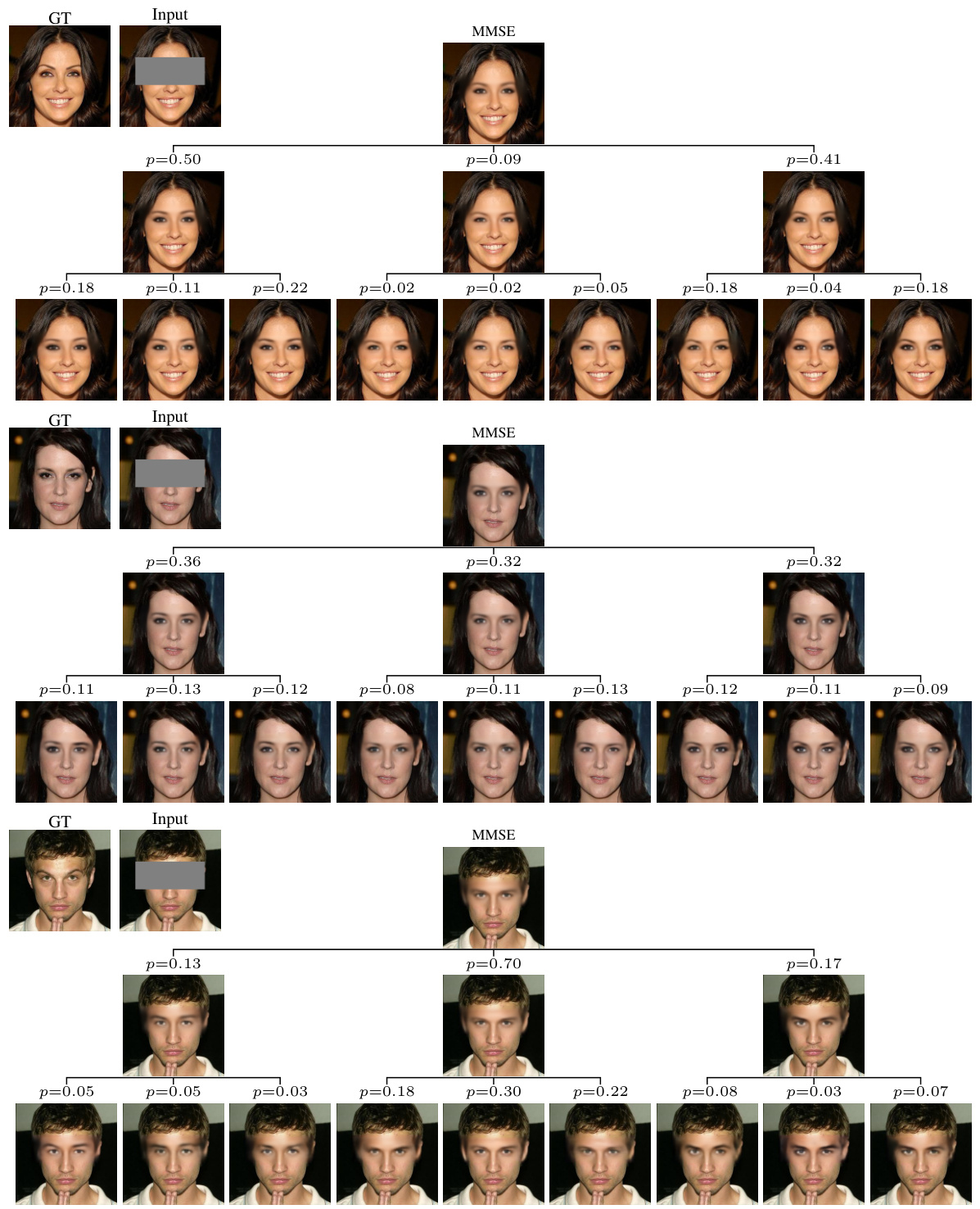
🔼 This figure shows a hierarchical decomposition of the minimum mean squared error (MMSE) predictor into prototypes for the task of mouth inpainting. The model predicts a tree structure where each node represents a cluster of plausible solutions, and each branch represents the probability of transitioning between clusters. The tree explores various options for mouth appearance, including lip size, mouth shape, and jawline shape, providing a hierarchical and probabilistic representation of the uncertainty in the inpainting task.
read the caption
Figure 1: Hierarchical decomposition of the minimum-MSE predictor into prototypes in the task of mouth inpainting. The predicted tree explores the different options of bigger/smaller lips, mouth opening/closing, round/square jawline, etc.
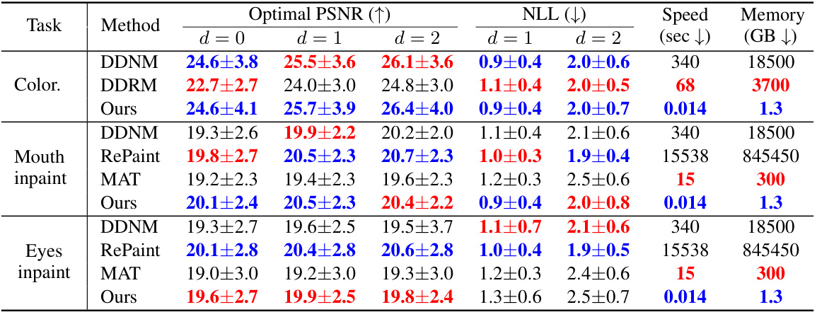
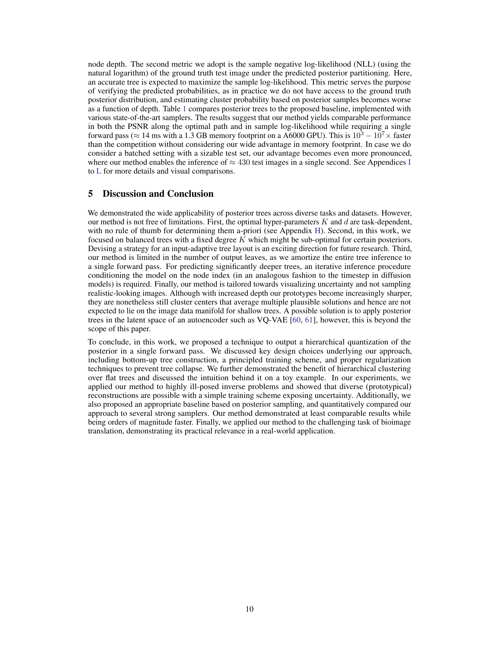
🔼 This table compares the proposed method’s performance against a baseline method on the FFHQ dataset for three different image inpainting tasks. The baseline uses hierarchical K-means clustering on 100 posterior samples per image. The table presents quantitative results including optimal Peak Signal-to-Noise Ratio (PSNR) at different tree depths (d=0,1,2), negative log-likelihood (NLL) (omitting the trivial root node), forward pass speed, and memory usage (for a single test image inference on an A6000 GPU). Blue and red highlight the best and second-best performing methods for each task and metric.
read the caption
Table 1: Comparison to the proposed baseline on 100 test images from the FFHQ dataset. Hierarchical K-means was applied to 100 posterior samples per test image. Runtime is reported as both the speed of a forward pass (sec) and the memory usage (GB) required to infer a single test image with a batch of 1 on an A6000 GPU. The NLL at the root node (d = 0) is trivial and therefore omitted. Blue and Red indicate best and second best respectively.
In-depth insights#
Hierarchical Uncertainty#
Hierarchical uncertainty, in the context of this research paper, likely refers to a method of representing and exploring uncertainty in a multi-level, tree-structured format. Instead of presenting a single prediction, the model outputs a tree where each node encapsulates a cluster of possible solutions at a particular level of granularity, and each branch represents a different hypothesis about the underlying solution. This hierarchical approach allows for a more nuanced representation of uncertainty, providing insights into the multiple modes and their relative probabilities that a flat representation might miss. It makes exploration more tractable for high-dimensional data (such as images) by providing a structured way to navigate the uncertainty space. The effectiveness is highlighted by the method’s ability to balance the need for providing a concise summary of the posterior with the capacity to fully reflect the complexities of multi-modal solutions. The speed and efficiency of the hierarchical approach are also emphasized, showing a significant performance improvement over traditional diffusion-based methods. Overall, the proposed method presents a potentially powerful new tool for representing and communicating uncertainty in image processing, offering greater speed and interpretability than existing techniques.
Posterior Tree Modeling#
Posterior tree modeling presents a novel approach to visualizing high-dimensional posterior distributions, a common challenge in inverse problems. Instead of relying on point estimates or numerous samples, it uses a feedforward neural network to predict a tree structure summarizing the posterior. This hierarchical representation allows users to explore uncertainty at different granularities, starting with a high-level overview and gradually drilling down to finer details. The tree’s nodes represent clusters of likely solutions, and the branches indicate their probabilities. This makes it easier for users to grasp complex uncertainty landscapes compared to traditional methods. The key advantage is the speed; this approach is far faster than methods based on posterior sampling. Uncertainty quantification is improved by explicitly representing multiple modes, leading to a richer understanding of plausible solutions. However, the optimal tree structure’s depth and width remain to be investigated further, potentially limiting generalizability. More investigation into these hyperparameters could enhance the approach’s flexibility and usefulness across diverse applications.
Diverse Inverse Problems#
A study on diverse inverse problems would explore the application of different mathematical and computational techniques to a wide range of problems where the goal is to infer unobserved variables from indirect measurements. The core challenge in inverse problems lies in their ill-posed nature – the solution may not be unique or may be highly sensitive to noise in the measurements. Addressing this challenge necessitates sophisticated methods to regularize the problem, leverage prior knowledge, or incorporate probabilistic models. A truly diverse study would include examples from various fields, such as image processing (e.g., deblurring, inpainting, super-resolution), medical imaging (e.g., MRI, CT reconstruction), geophysics (e.g., seismic inversion), and remote sensing. The focus would be on comparing and contrasting the effectiveness of different methodologies across diverse problem types, and considering the relative importance of factors like data quality, computational cost, and prior information. The research would likely highlight common themes and challenges, potentially leading to new algorithms or frameworks for solving inverse problems in a more general and robust manner. A key aspect would involve thorough analysis of uncertainty quantification techniques, which are vital for interpreting the results in ill-posed scenarios. This is a wide ranging research topic with significant potential.
Speed and Efficiency#
The speed and efficiency of the proposed method are crucial aspects of the research. The authors highlight that their approach achieves comparable performance to existing, more computationally expensive methods but with significantly faster execution times. This enhanced efficiency is a major advantage, enabling quicker analysis and visualization of complex, high-dimensional posterior distributions. Orders of magnitude greater speed is reported in comparison to a baseline hierarchical clustering technique that samples from a diffusion-based posterior, emphasizing the practical benefits for real-world applications. The speed advantage stems from a clever tree-structured prediction approach using a single forward pass of a neural network, avoiding the multi-step sampling procedures of baseline methods. This efficiency enables the processing of numerous inputs rapidly, which is particularly important in time-sensitive applications and for datasets with substantial amounts of data. The method’s scalability and speed are compelling arguments for its broader adoption.
Future Research#
Future research directions stemming from this work on hierarchical uncertainty exploration using feedforward posterior trees could involve several key areas. Improving the efficiency of tree inference for deeper trees is crucial, potentially through iterative inference methods conditioned on node indices, similar to diffusion models. Exploring input-adaptive tree layouts that dynamically adjust tree depth and width based on input complexity would enhance the method’s versatility. Investigating the use of alternative association measures beyond MSE loss, such as perceptual metrics, could tailor the approach to specific application needs. Additionally, research could focus on developing techniques to generate more realistic samples from the resulting posterior tree clusters, rather than simply using cluster centers as representations. Finally, extending the method to handle higher-dimensional data and exploring its applications in diverse fields beyond imaging is a promising avenue for future work. Overall, the potential of the proposed posterior trees and its adaptability warrant further investigation and refinement.
More visual insights#
More on figures

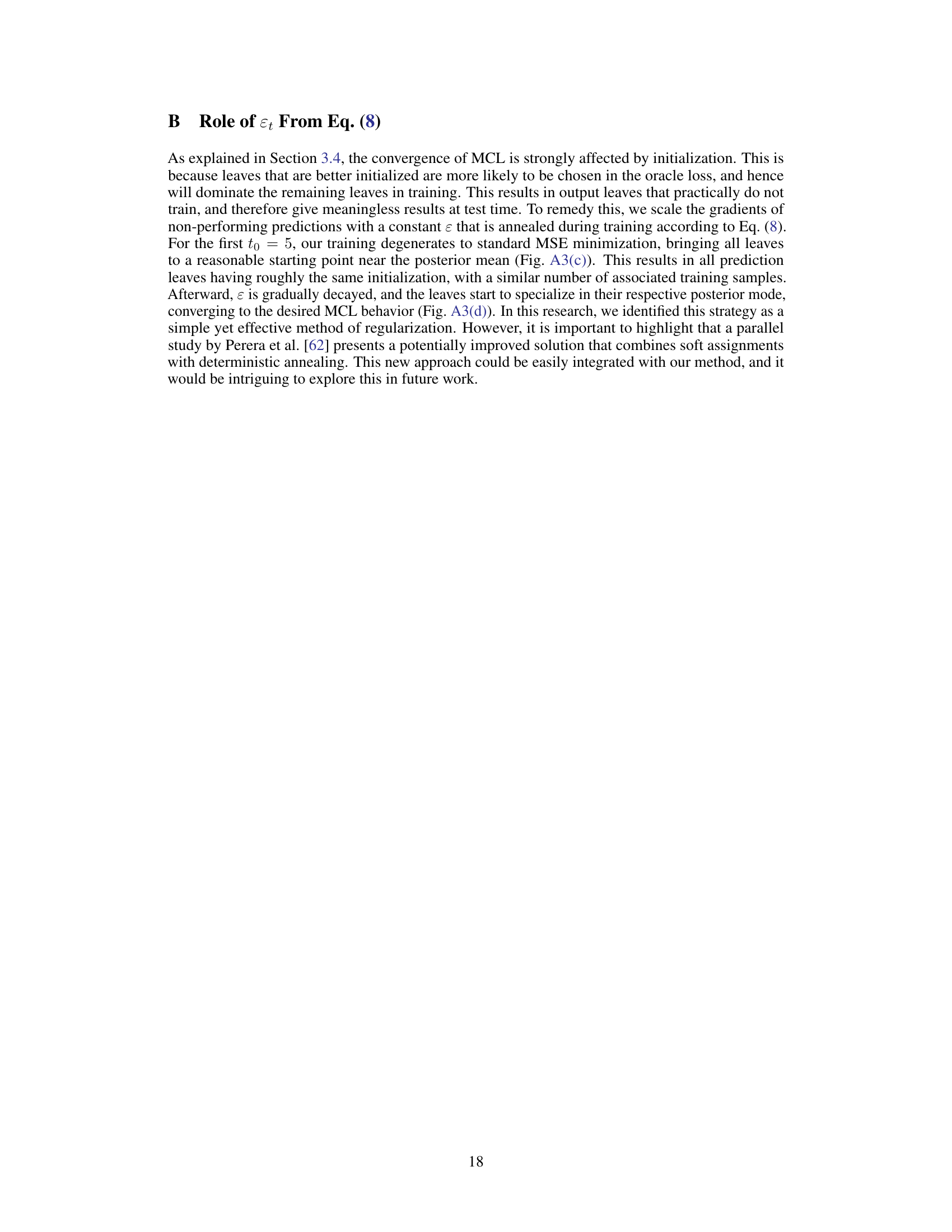
🔼 This figure illustrates the method’s architecture and training process. The model takes a degraded input image (y) and produces Kd leaf predictions (bottom-level nodes of the tree) and their associated probabilities. It iteratively builds a tree from the bottom-up, combining predictions at each level based on weighted averaging. During training, it starts from the root node (the minimum MSE prediction) and propagates the ground truth (x) down the tree, comparing it to its immediate children and accumulating a loss based on the MSE.
read the caption
Figure 2: Method overview. Our model T(y; θ) receives a degraded image y and predicts {xk1,...,kak1,...,kd=1, the bottom Kd leaves, and their probabilities {αk1,...,kak1,...,kd=1 (faint blue box; illustrated here for K = 3 and d = 2). Next, the tree is iteratively constructed from the bottom up using weighted averaging, until we reach the root node which is the minimum MSE predictor xMMSE. During training, starting from the root, the ground truth x is propagated through the tree until it reaches the leaves (dashed red lines). At tree level d, x is compared to its immediate K children nodes, and the MSE loss to the nearest child is added to the loss trajectory.

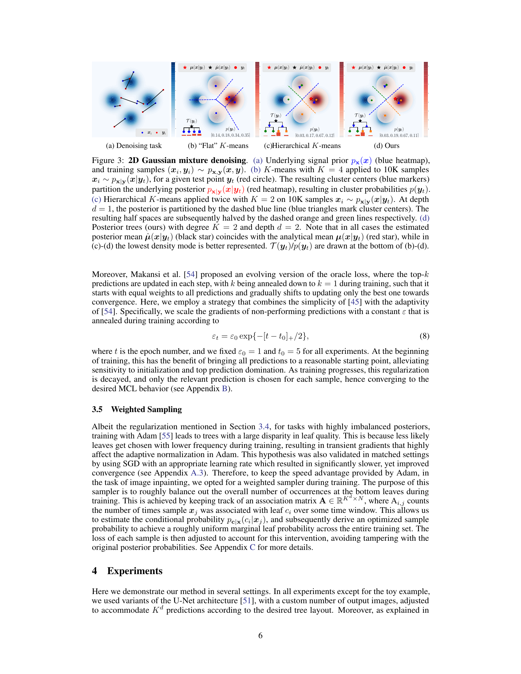
🔼 This figure shows a comparison of different methods for visualizing the posterior distribution in a 2D Gaussian mixture denoising task. It compares standard K-means, hierarchical K-means, and the proposed ‘Posterior Trees’ method. The figure illustrates how each method partitions the posterior distribution and estimates cluster probabilities, highlighting the advantages of the hierarchical approach in representing multi-modal posteriors.
read the caption
Figure 3: 2D Gaussian mixture denoising. (a) Underlying signal prior px(x) (blue heatmap), and training samples (xi, Yi) ~ Px,y(x, y). (b) K-means with K = 4 applied to 10K samples Xi ~Pxy(xYt), for a given test point yt (red circle). The resulting cluster centers (blue markers) partition the underlying posterior px|y (xyt) (red heatmap), resulting in cluster probabilities p(yt). (c) Hierarchical K-means applied twice with K = 2 on 10K samples xi ~ Px|y(X|Yt). At depth d = 1, the posterior is partitioned by the dashed blue line (blue triangles mark cluster centers). The resulting half spaces are subsequently halved by the dashed orange and green lines respectively. (d) Posterior trees (ours) with degree K = 2 and depth d = 2. Note that in all cases the estimated posterior mean (x|yt) (black star) coincides with the analytical mean μ(x|yt) (red star), while in (c)-(d) the lowest density mode is better represented. T(yt)/p(yt) are drawn at the bottom of (b)-(d).

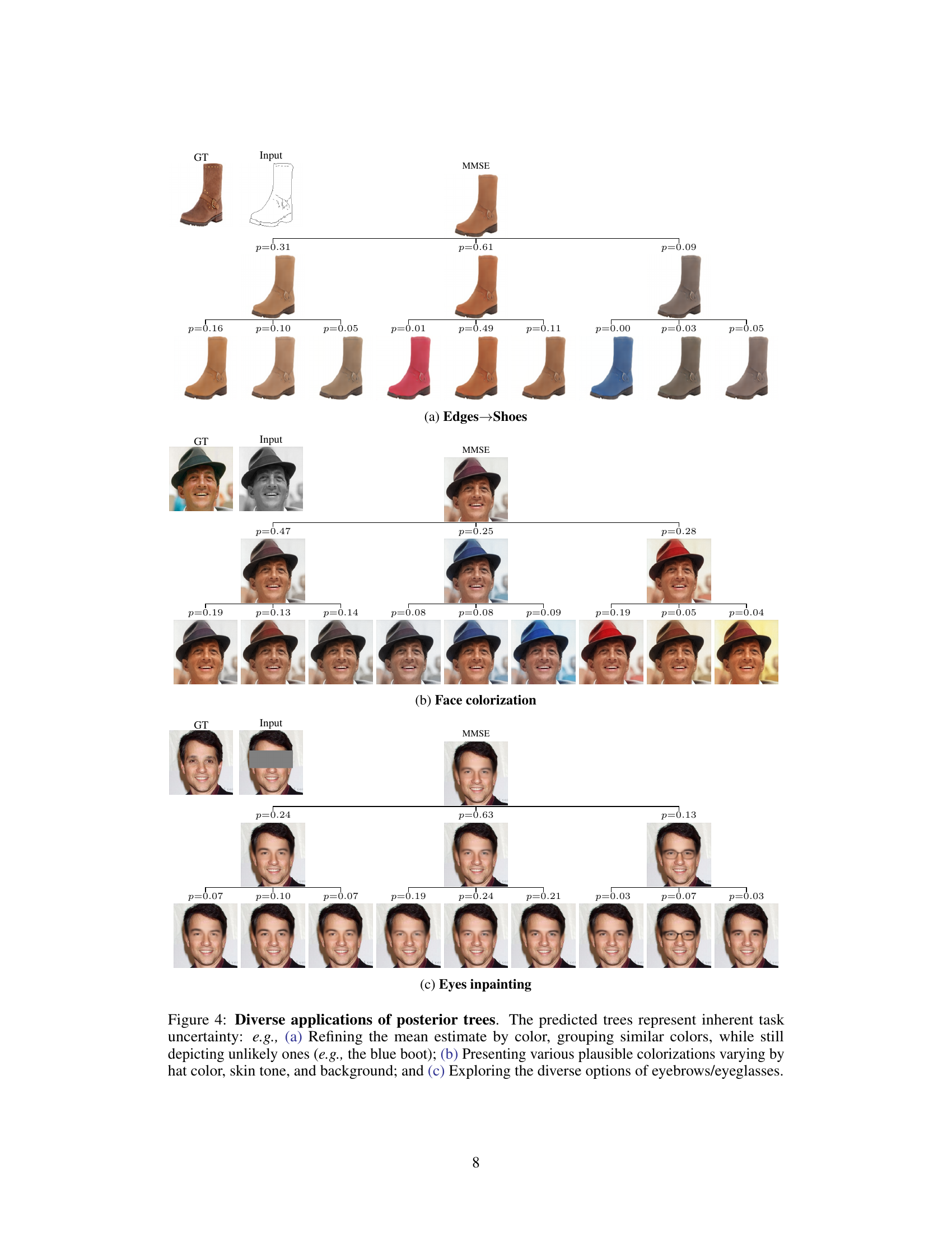
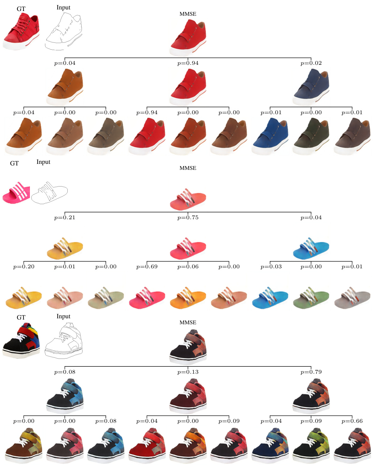
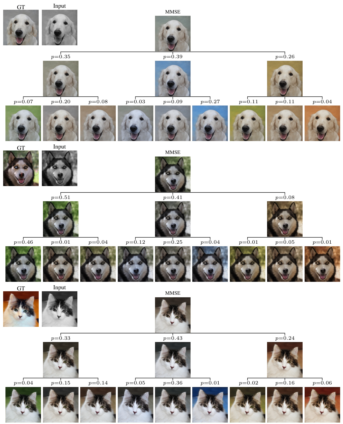
🔼 This figure demonstrates the application of posterior trees to three different image restoration tasks: Edges to Shoes, Face Colorization, and Eyes Inpainting. Each row shows a different task, with the input image on the left, the minimum mean squared error (MMSE) estimate in the center, and a tree representing the hierarchical decomposition of the posterior distribution on the right. The leaves of the tree show diverse and plausible solutions. This demonstrates the ability of the method to handle different kinds of uncertainty in diverse tasks.
read the caption
Figure 4: Diverse applications of posterior trees. The predicted trees represent inherent task uncertainty: e.g., (a) Refining the mean estimate by color, grouping similar colors, while still depicting unlikely ones (e.g., the blue boot); (b) Presenting various plausible colorizations varying by hat color, skin tone, and background; and (c) Exploring the diverse options of eyebrows/eyeglasses.
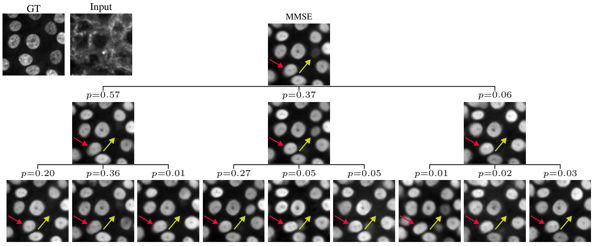
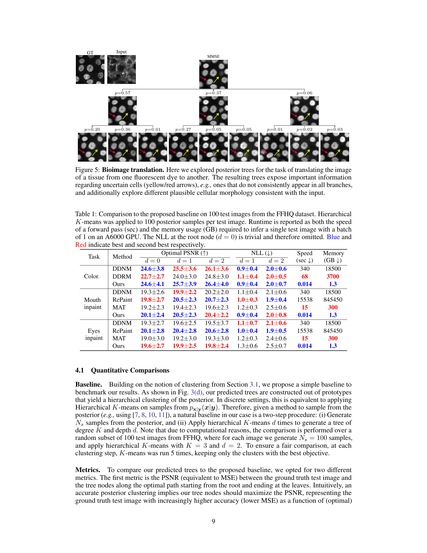
🔼 This figure shows an example of applying the Posterior Trees method to a bioimage translation task. The input is a microscopy image of cells stained with one fluorescent dye, and the goal is to predict what the image would look like if stained with a different fluorescent dye. The figure shows the results of the prediction, where the tree structure represents different possible interpretations of the image, with the probabilities of each interpretation shown on the branches. The red and yellow arrows highlight cells where the uncertainty is particularly high. The results demonstrate the ability of the method to quantify and communicate uncertainty, and to explore the space of plausible solutions in a visually intuitive way.
read the caption
Figure 5: Bioimage translation. Here we explored posterior trees for the task of translating the image of a tissue from one fluorescent dye to another. The resulting trees expose important information regarding uncertain cells (yellow/red arrows), e.g., ones that do not consistently appear in all branches, and additionally explore different plausible cellular morphology consistent with the input.
🔼 This figure shows a hierarchical decomposition of the minimum mean squared error (MSE) predictor for mouth inpainting. The model predicts a tree structure, where each branch represents a plausible solution (e.g., different lip sizes or shapes) with an associated probability. This tree visualization helps users explore the uncertainty associated with the prediction, offering various plausible options instead of a single reconstruction.
read the caption
Figure 1: Hierarchical decomposition of the minimum-MSE predictor into prototypes in the task of mouth inpainting. The predicted tree explores the different options of bigger/smaller lips, mouth opening/closing, round/square jawline, etc.

🔼 This figure shows the overall method used in the paper. The model receives a degraded image as input and predicts Kd leaves and their probabilities. Then it constructs a tree from bottom up using weighted averaging until it reaches the root node which is the minimum MSE predictor. During training, the ground truth is propagated through the tree to reach the leaves and the MSE loss is compared with its children nodes.
read the caption
Figure 2: Method overview. Our model T(y; θ) receives a degraded image y and predicts {xk1,...,kak1,...,ka=1, the bottom Kd leaves, and their probabilities {αk1,...,ka}k1,...,ka=1 (faint blue box; illustrated here for K = 3 and d = 2). Next, the tree is iteratively constructed from the bottom up using weighted averaging, until we reach the root node which is the minimum MSE predictor xMMSE. During training, starting from the root, the ground truth x is propagated through the tree until it reaches the leaves (dashed red lines). At tree level d, x is compared to its immediate K children nodes, and the MSE loss to the nearest child is added to the loss trajectory.
🔼 This figure demonstrates the comparison of different methods for denoising a 2D Gaussian mixture. It shows how K-means, hierarchical K-means, and the proposed method (posterior trees) partition the posterior distribution and visualize the uncertainty. The figure highlights that the proposed method better represents the lower-density modes compared to the other methods.
read the caption
Figure 3: 2D Gaussian mixture denoising. (a) Underlying signal prior px(x) (blue heatmap), and training samples (xi, Yi) ~ Px,y(x, y). (b) K-means with K = 4 applied to 10K samples xi ~Pxy(xYt), for a given test point yt (red circle). The resulting cluster centers (blue markers) partition the underlying posterior px|y (xyt) (red heatmap), resulting in cluster probabilities p(yt). (c) Hierarchical K-means applied twice with K = 2 on 10K samples xi ~ Px|y(X|Yt). At depth d = 1, the posterior is partitioned by the dashed blue line (blue triangles mark cluster centers). The resulting half spaces are subsequently halved by the dashed orange and green lines respectively. (d) Posterior trees (ours) with degree K = 2 and depth d = 2. Note that in all cases the estimated posterior mean (x|yt) (black star) coincides with the analytical mean μ(x|yt) (red star), while in (c)-(d) the lowest density mode is better represented. T(yt)/p(yt) are drawn at the bottom of (b)-(d).

🔼 This figure shows a comparison of different methods for visualizing uncertainty in a 2D Gaussian mixture denoising task. It compares standard K-means, hierarchical K-means, and the proposed ‘Posterior Trees’ method. Each method’s ability to capture the underlying posterior distribution, including multiple modes, is visualized. The figure highlights that the proposed Posterior Trees method effectively visualizes the uncertainty across multiple levels of granularity.
read the caption
Figure 3: 2D Gaussian mixture denoising. (a) Underlying signal prior px(x) (blue heatmap), and training samples (xi, Yi) ~ Px,y(x, y). (b) K-means with K = 4 applied to 10K samples Xi ~Pxy(xYt), for a given test point yt (red circle). The resulting cluster centers (blue markers) partition the underlying posterior px|y (xyt) (red heatmap), resulting in cluster probabilities p(yt). (c) Hierarchical K-means applied twice with K = 2 on 10K samples xi ~ Px|y(X|Yt). At depth d = 1, the posterior is partitioned by the dashed blue line (blue triangles mark cluster centers). The resulting half spaces are subsequently halved by the dashed orange and green lines respectively. (d) Posterior trees (ours) with degree K = 2 and depth d = 2. Note that in all cases the estimated posterior mean (x|yt) (black star) coincides with the analytical mean μ(x|yt) (red star), while in (c)-(d) the lowest density mode is better represented. T(yt)/p(yt) are drawn at the bottom of (b)-(d).

🔼 This figure compares different methods for visualizing the posterior distribution of a 2D Gaussian mixture model. It shows the underlying signal prior, the results of applying K-means, hierarchical K-means, and the proposed method (Posterior Trees). The figure highlights how the proposed method effectively captures multimodality and uncertainty in the posterior.
read the caption
Figure 3: 2D Gaussian mixture denoising. (a) Underlying signal prior px(x) (blue heatmap), and training samples (xi, Yi) ~ Px,y(x, y). (b) K-means with K = 4 applied to 10K samples xi ~ Pxy(xYt), for a given test point yt (red circle). The resulting cluster centers (blue markers) partition the underlying posterior px|y (xyt) (red heatmap), resulting in cluster probabilities p(yt). (c) Hierarchical K-means applied twice with K = 2 on 10K samples xi ~ Px|y(X|Yt). At depth d = 1, the posterior is partitioned by the dashed blue line (blue triangles mark cluster centers). The resulting half spaces are subsequently halved by the dashed orange and green lines respectively. (d) Posterior trees (ours) with degree K = 2 and depth d = 2. Note that in all cases the estimated posterior mean (x|yt) (black star) coincides with the analytical mean μ(x|yt) (red star), while in (c)-(d) the lowest density mode is better represented. T(yt)/p(yt) are drawn at the bottom of (b)-(d).
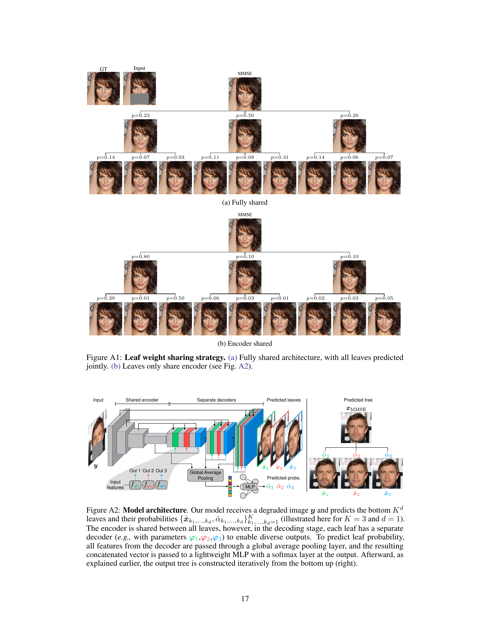
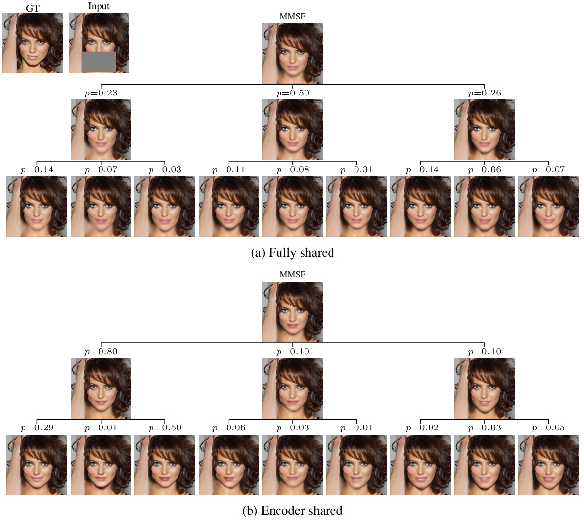
🔼 This figure compares two different architectures for the proposed method, which is called ‘posterior trees’. Both architectures use a U-Net, but differ in how they share parameters across leaves of the tree. The fully shared architecture (a) shares parameters across all leaves, potentially leading to less diversity in the predictions. The encoder shared architecture (b) only shares the encoder part of the U-Net, leading to separate decoder parameters for each leaf. This approach balances between computational efficiency and prediction diversity, which is crucial for accurately representing multi-modal posterior distributions.
read the caption
Figure A1: Leaf weight sharing strategy. (a) Fully shared architecture, with all leaves predicted jointly. (b) Leaves only share encoder (see Fig. A2).

🔼 This figure compares different methods for visualizing the posterior distribution of a 2D Gaussian mixture model. It shows how K-means clustering (flat and hierarchical) and the proposed ‘Posterior Trees’ method perform in capturing the multi-modal nature of the posterior. The figure highlights that the hierarchical methods, especially the proposed approach, better represent low-density modes in the posterior.
read the caption
Figure 3: 2D Gaussian mixture denoising. (a) Underlying signal prior px(x) (blue heatmap), and training samples (xi, Yi) ~ Px,y(x, y). (b) K-means with K = 4 applied to 10K samples xi ~ Pxy(xYt), for a given test point yt (red circle). The resulting cluster centers (blue markers) partition the underlying posterior px|y (xyt) (red heatmap), resulting in cluster probabilities p(yt). (c) Hierarchical K-means applied twice with K = 2 on 10K samples xi ~ Px|y(X|Yt). At depth d = 1, the posterior is partitioned by the dashed blue line (blue triangles mark cluster centers). The resulting half spaces are subsequently halved by the dashed orange and green lines respectively. (d) Posterior trees (ours) with degree K = 2 and depth d = 2. Note that in all cases the estimated posterior mean (x|yt) (black star) coincides with the analytical mean μ(x|yt) (red star), while in (c)-(d) the lowest density mode is better represented. T(yt)/p(yt) are drawn at the bottom of (b)-(d).

🔼 This figure demonstrates the results of applying different clustering methods to a 2D Gaussian mixture denoising task. It compares K-means, hierarchical K-means, and the proposed posterior trees method. The results show how the different methods partition the posterior distribution and their strengths and weaknesses in representing the underlying modes, especially low-density modes.
read the caption
Figure 3: 2D Gaussian mixture denoising. (a) Underlying signal prior px(x) (blue heatmap), and training samples (xi, Yi) ~ Px,y(x, y). (b) K-means with K = 4 applied to 10K samples Xi ~Pxy(xYt), for a given test point yt (red circle). The resulting cluster centers (blue markers) partition the underlying posterior px|y (xyt) (red heatmap), resulting in cluster probabilities p(yt). (c) Hierarchical K-means applied twice with K = 2 on 10K samples xi ~ Px|y(X|Yt). At depth d = 1, the posterior is partitioned by the dashed blue line (blue triangles mark cluster centers). The resulting half spaces are subsequently halved by the dashed orange and green lines respectively. (d) Posterior trees (ours) with degree K = 2 and depth d = 2. Note that in all cases the estimated posterior mean (x|yt) (black star) coincides with the analytical mean μ(x|yt) (red star), while in (c)-(d) the lowest density mode is better represented. T(yt)/p(yt) are drawn at the bottom of (b)-(d).
🔼 This figure shows an example of how the model predicts a tree-structured representation of the posterior distribution for a mouth inpainting task. The root node represents the minimum mean squared error (MMSE) prediction, which is a single image. However, the model also predicts a tree where each branch represents a plausible alternative reconstruction (e.g., different lip sizes and shapes, mouth openness), with associated probabilities. This hierarchical structure helps visualize uncertainty across multiple levels of granularity.
read the caption
Figure 1: Hierarchical decomposition of the minimum-MSE predictor into prototypes in the task of mouth inpainting. The predicted tree explores the different options of bigger/smaller lips, mouth opening/closing, round/square jawline, etc.
🔼 This figure shows a comparison of different methods for visualizing the posterior distribution of a 2D Gaussian mixture denoising task. It compares the results of K-means clustering, hierarchical K-means clustering, and the proposed ‘Posterior Trees’ method. The figure highlights how the proposed method effectively captures multi-modal aspects of the posterior distribution, representing both high- and low-density regions more accurately than simpler clustering techniques.
read the caption
Figure 3: 2D Gaussian mixture denoising. (a) Underlying signal prior px(x) (blue heatmap), and training samples (xi, Yi) ~ Px,y(x, y). (b) K-means with K = 4 applied to 10K samples xi ~ Pxy(xYt), for a given test point yt (red circle). The resulting cluster centers (blue markers) partition the underlying posterior px|y (xyt) (red heatmap), resulting in cluster probabilities p(yt). (c) Hierarchical K-means applied twice with K = 2 on 10K samples xi ~ Px|y(X|Yt). At depth d = 1, the posterior is partitioned by the dashed blue line (blue triangles mark cluster centers). The resulting half spaces are subsequently halved by the dashed orange and green lines respectively. (d) Posterior trees (ours) with degree K = 2 and depth d = 2. Note that in all cases the estimated posterior mean (x|yt) (black star) coincides with the analytical mean μ(x|yt) (red star), while in (c)-(d) the lowest density mode is better represented. T(yt)/p(yt) are drawn at the bottom of (b)-(d).

🔼 The figure shows a hierarchical decomposition of the minimum mean squared error (MMSE) predictor into prototypes for mouth inpainting. The predicted tree structure visually represents multiple plausible solutions (prototypes) and their probabilities, branching out to explore variations in lip size, mouth shape, and jawline. This illustrates how the model captures uncertainty by providing not just a single best guess, but a range of possibilities.
read the caption
Figure 1: Hierarchical decomposition of the minimum-MSE predictor into prototypes in the task of mouth inpainting. The predicted tree explores the different options of bigger/smaller lips, mouth opening/closing, round/square jawline, etc.

🔼 This figure compares the results of three different methods for image colorization: DDNM, DDRM, and the proposed method. Each method’s results are presented as a tree, where the root node is the minimum MSE predictor (MMSE) and the leaf nodes are the different colorized images. The probabilities of each leaf node are also shown. The figure demonstrates that the proposed method produces more diverse and higher-quality results compared to the baselines.
read the caption
Figure A11: Tree comparison in colorization.

🔼 This figure compares the results of different posterior sampling methods with the proposed method for the task of mouth inpainting. The different methods are compared in terms of the generated samples and their respective probabilities. The proposed method shows a better representation of the underlying uncertainty by providing a more diverse set of samples.
read the caption
Figure A12: Tree comparison in mouth inpainting.

🔼 This figure demonstrates the 2D Gaussian mixture denoising task. It compares different methods for visualizing the posterior distribution: K-means, hierarchical K-means, and the proposed posterior trees method. The results show that the posterior trees method effectively visualizes the uncertainty in the posterior distribution across multiple levels of granularity.
read the caption
Figure 3: 2D Gaussian mixture denoising. (a) Underlying signal prior px(x) (blue heatmap), and training samples (xi, Yi) ~ Px,y(x, y). (b) K-means with K = 4 applied to 10K samples xi ~ Pxy(xYt), for a given test point yt (red circle). The resulting cluster centers (blue markers) partition the underlying posterior px|y (xyt) (red heatmap), resulting in cluster probabilities p(yt). (c) Hierarchical K-means applied twice with K = 2 on 10K samples xi ~ Px|y(X|Yt). At depth d = 1, the posterior is partitioned by the dashed blue line (blue triangles mark cluster centers). The resulting half spaces are subsequently halved by the dashed orange and green lines respectively. (d) Posterior trees (ours) with degree K = 2 and depth d = 2. Note that in all cases the estimated posterior mean (x|yt) (black star) coincides with the analytical mean μ(x|yt) (red star), while in (c)-(d) the lowest density mode is better represented. T(yt)/p(yt) are drawn at the bottom of (b)-(d).
🔼 This figure shows a hierarchical decomposition of the minimum mean squared error (MMSE) predictor into prototypes for the task of mouth inpainting. The inpainting task is inherently ambiguous, and the posterior distribution contains many plausible solutions. The figure shows a tree structure, where each node represents a set of similar inpainted images, and the probabilities at each node represent the likelihood of each branch. The tree structure allows for efficient exploration of the uncertainty in the predictions, allowing a user to see different inpainting options (e.g., bigger/smaller lips, mouth opening/closing, jawline shapes) and their probabilities.
read the caption
Figure 1: Hierarchical decomposition of the minimum-MSE predictor into prototypes in the task of mouth inpainting. The predicted tree explores the different options of bigger/smaller lips, mouth opening/closing, round/square jawline, etc.
🔼 This figure demonstrates the applications of posterior trees on different image tasks, including shoes inpainting, face colorization, and eyes inpainting. The results showcase how posterior trees effectively capture and represent uncertainty by providing multiple plausible predictions at different levels of granularity.
read the caption
Figure 4: Diverse applications of posterior trees. The predicted trees represent inherent task uncertainty: e.g., (a) Refining the mean estimate by color, grouping similar colors, while still depicting unlikely ones (e.g., the blue boot); (b) Presenting various plausible colorizations varying by hat color, skin tone, and background; and (c) Exploring the diverse options of eyebrows/eyeglasses.
🔼 This figure demonstrates the results of 2D Gaussian mixture denoising using different methods: K-means, hierarchical K-means, and the proposed posterior trees. It shows how each method partitions the posterior distribution and estimates cluster probabilities, highlighting the advantages of the hierarchical approach in representing multi-modal posteriors.
read the caption
Figure 3: 2D Gaussian mixture denoising. (a) Underlying signal prior px(x) (blue heatmap), and training samples (xi, Yi) ~ Px,y(x, y). (b) K-means with K = 4 applied to 10K samples xi ~ Px|y(x|Yt), for a given test point yt (red circle). The resulting cluster centers (blue markers) partition the underlying posterior px|y (x|yt) (red heatmap), resulting in cluster probabilities p(yt). (c) Hierarchical K-means applied twice with K = 2 on 10K samples xi ~ Px|y(x|Yt). At depth d = 1, the posterior is partitioned by the dashed blue line (blue triangles mark cluster centers). The resulting half spaces are subsequently halved by the dashed orange and green lines respectively. (d) Posterior trees (ours) with degree K = 2 and depth d = 2. Note that in all cases the estimated posterior mean (x|yt) (black star) coincides with the analytical mean μ(x|yt) (red star), while in (c)-(d) the lowest density mode is better represented. T(yt)/p(yt) are drawn at the bottom of (b)-(d).

🔼 This figure shows a hierarchical decomposition of the minimum mean squared error (MMSE) predictor for mouth inpainting. The prediction is not a single image, but a tree where each branch represents a different plausible reconstruction of the mouth, with associated probabilities. The tree structure allows for exploring different variations in lip size, mouth shape, and jawline, providing a more comprehensive understanding of the uncertainty in the prediction than a single MMSE estimate would allow.
read the caption
Figure 1: Hierarchical decomposition of the minimum-MSE predictor into prototypes in the task of mouth inpainting. The predicted tree explores the different options of bigger/smaller lips, mouth opening/closing, round/square jawline, etc.

🔼 This figure shows three examples of how posterior trees can be applied to different image tasks. In each case, the predicted tree reveals multiple plausible solutions (represented as images) and their likelihoods (represented as probabilities). (a) shows edge-to-shoe generation, illustrating how the tree encompasses a range of color variations. (b) demonstrates face colorization, with the tree exploring different possibilities for skin tones, hats, and backgrounds. Finally, (c) illustrates eye inpainting, showcasing variations in eye opening, eyebrows, and the presence/absence of glasses. In essence, it highlights the tree’s utility in representing various solutions and their probability.
read the caption
Figure 4: Diverse applications of posterior trees. The predicted trees represent inherent task uncertainty: e.g., (a) Refining the mean estimate by color, grouping similar colors, while still depicting unlikely ones (e.g., the blue boot); (b) Presenting various plausible colorizations varying by hat color, skin tone, and background; and (c) Exploring the diverse options of eyebrows/eyeglasses.
🔼 This figure shows a hierarchical decomposition of the minimum mean squared error (MSE) predictor into prototypes for the task of mouth inpainting. The model predicts a tree structure where each node represents a cluster of similar mouth shapes, and the branches represent the probability of transitioning between different mouth configurations. This tree allows for exploration of the different possible solutions for mouth inpainting, ranging from smaller or larger lips, different degrees of mouth opening or closing, and various jawline shapes. The probability of each path (combination of choices down the tree) reflects the relative likelihood of the corresponding mouth configuration given the input image.
read the caption
Figure 1: Hierarchical decomposition of the minimum-MSE predictor into prototypes in the task of mouth inpainting. The predicted tree explores the different options of bigger/smaller lips, mouth opening/closing, round/square jawline, etc.

🔼 This figure compares different methods for visualizing uncertainty in a 2D Gaussian mixture denoising task. It shows the underlying signal distribution, results from K-means clustering (both flat and hierarchical), and the results from the proposed ‘posterior trees’ method. The comparison highlights how the posterior trees method effectively visualizes the posterior distribution across multiple levels of granularity, capturing even low-density modes.
read the caption
Figure 3: 2D Gaussian mixture denoising. (a) Underlying signal prior px(x) (blue heatmap), and training samples (xi, Yi) ~ Px,y(x, y). (b) K-means with K = 4 applied to 10K samples Xi ~Pxy(xYt), for a given test point yt (red circle). The resulting cluster centers (blue markers) partition the underlying posterior px|y (xyt) (red heatmap), resulting in cluster probabilities p(yt). (c) Hierarchical K-means applied twice with K = 2 on 10K samples xi ~ Px|y(X|Yt). At depth d = 1, the posterior is partitioned by the dashed blue line (blue triangles mark cluster centers). The resulting half spaces are subsequently halved by the dashed orange and green lines respectively. (d) Posterior trees (ours) with degree K = 2 and depth d = 2. Note that in all cases the estimated posterior mean (x|yt) (black star) coincides with the analytical mean μ(x|yt) (red star), while in (c)-(d) the lowest density mode is better represented. T(yt)/p(yt) are drawn at the bottom of (b)-(d).
Full paper#
