TL;DR#
Brain-machine interfaces (BMIs) hold immense potential for restoring motor function in paralyzed individuals. However, current state-of-the-art deep learning BMIs are ‘black boxes,’ raising safety concerns. Explainable models like the Kalman filter offer safety but compromise performance.
This research introduces KalmanNet, a hybrid BMI decoder that combines the strengths of both approaches. KalmanNet uses recurrent neural networks to augment Kalman filtering, creating a dynamic balance between reliance on brain activity and a dynamical model. The results demonstrate that KalmanNet matches or surpasses the performance of other deep-learning methods, while offering better interpretability and enhanced safety.
Key Takeaways#
Why does it matter?#
This paper is crucial for BMI researchers seeking to improve decoder performance while maintaining explainability. It bridges the gap between high-performing deep learning models and explainable traditional methods, offering a novel approach with potential for safer and more reliable BMI systems. The findings also highlight the importance of considering model generalization and robustness to noise in real-world applications. This work encourages future research into combining deep learning and traditional methods to increase performance while maintaining explainability and safety.
Visual Insights#
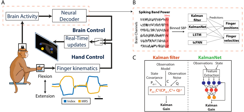
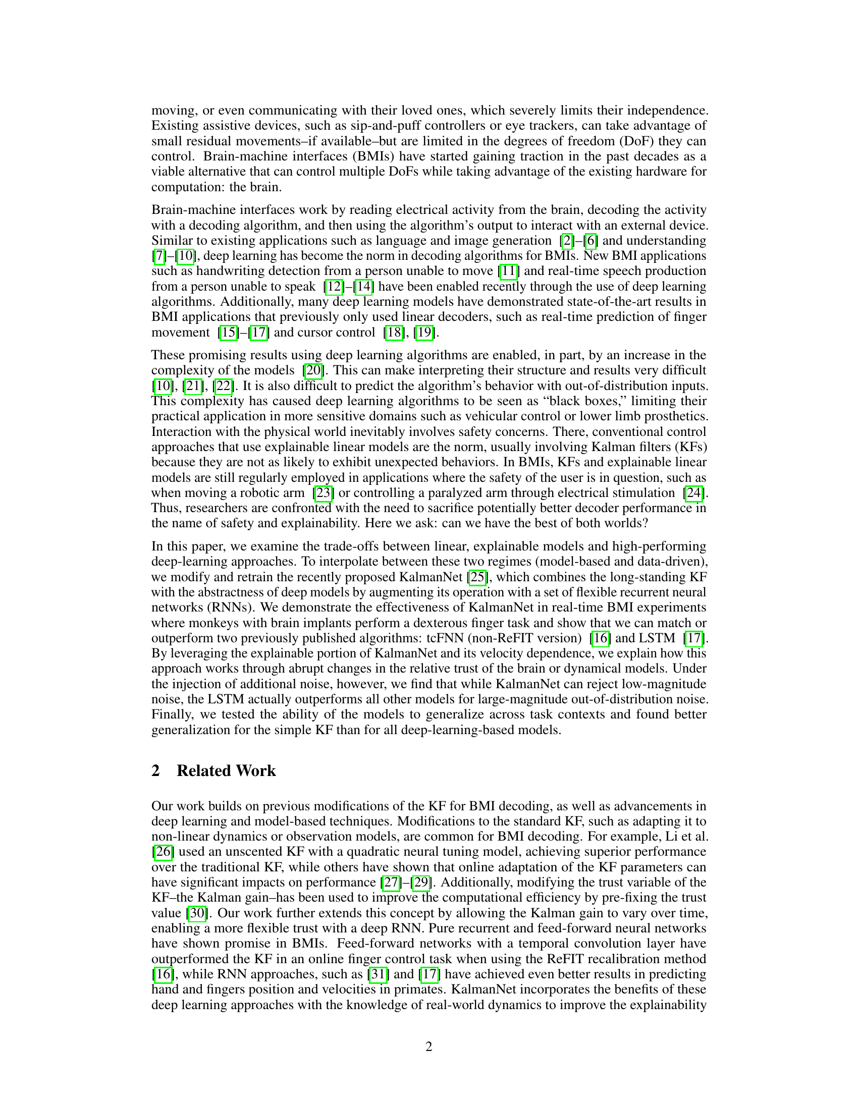
🔼 This figure provides a comprehensive overview of the experimental setup and the neural decoders used in the study. Panel A illustrates the task paradigm, showing a monkey performing a 2-DoF finger movement task under both brain control (using a neural decoder) and hand control. Panel B shows the signal processing pipeline for brain control trials, highlighting the extraction and binning of spiking band power (SBP) data. Finally, Panel C visually depicts the differences in Kalman gain computation between the traditional Kalman filter (KF) and KalmanNet, emphasizing KalmanNet’s use of recurrent neural networks.
read the caption
Figure 1: Task and Neural Decoders. (A) We trained a monkey to do a 2-DoF finger task (shown on screen) while brain activity and finger kinematics (index and middle-ring-small (MRS) traces shown below) are recorded. The monkey can do the task in hand control, using his hand, or in brain control. (B) In brain control, the SBP of each brain channel is extracted and binned every 50 milliseconds. Each neural decoder takes in a bin and predicts position and velocity, or only velocity. (C) The KF and KalmanNet differ in how they compute the Kalman gain: the KF uses the equation shown, while KalmanNet uses a set of RNNs.
In-depth insights#
Explainable BMI#
Explainable Brain-Machine Interfaces (BMIs) represent a crucial area of research focusing on the transparency and interpretability of BMI algorithms. Current state-of-the-art BMIs often leverage deep learning models, which, while powerful, are often considered “black boxes.” This lack of transparency poses significant challenges, especially in safety-critical applications where understanding the decision-making process is paramount. Explainable BMIs aim to address this by using models that provide insights into their predictions, enhancing trust and facilitating the detection of errors. Key methods involve incorporating elements of traditional control theory, such as Kalman filters, with neural networks, creating hybrid models that combine the strengths of both approaches. The balance between performance and explainability remains a major challenge, as simpler, more explainable models may sacrifice accuracy while highly complex models may lack transparency. Future work should focus on developing more robust and interpretable methods, potentially using techniques like model distillation or attention mechanisms, to further improve the balance between performance and interpretability in explainable BMIs. The ultimate goal is to develop BMIs that are not only effective but also trustworthy and safe for users.
KalmanNet Hybrid#
A KalmanNet hybrid system would integrate the strengths of Kalman filters and neural networks for improved performance and explainability in brain-machine interfaces (BMIs). Kalman filters provide a principled framework for incorporating prior knowledge about the system dynamics, leading to more robust and reliable predictions. However, they may struggle with complex, non-linear relationships. Neural networks excel at modeling these non-linear systems, but often lack interpretability. A hybrid architecture could leverage neural networks to learn complex relationships within the Kalman filter framework, potentially improving accuracy without sacrificing explainability. For example, the neural networks could be used to estimate model parameters or refine the Kalman gain dynamically based on observed data. The result would be a system that is both accurate and interpretable, addressing a critical need for safe and reliable BMIs. A key challenge is balancing the trade-off between model accuracy and interpretability. Overly complex neural network components could reduce interpretability, making the system susceptible to unexpected behavior. Careful design of the neural network architecture and training processes is essential to address this concern.
Offline/Online Results#
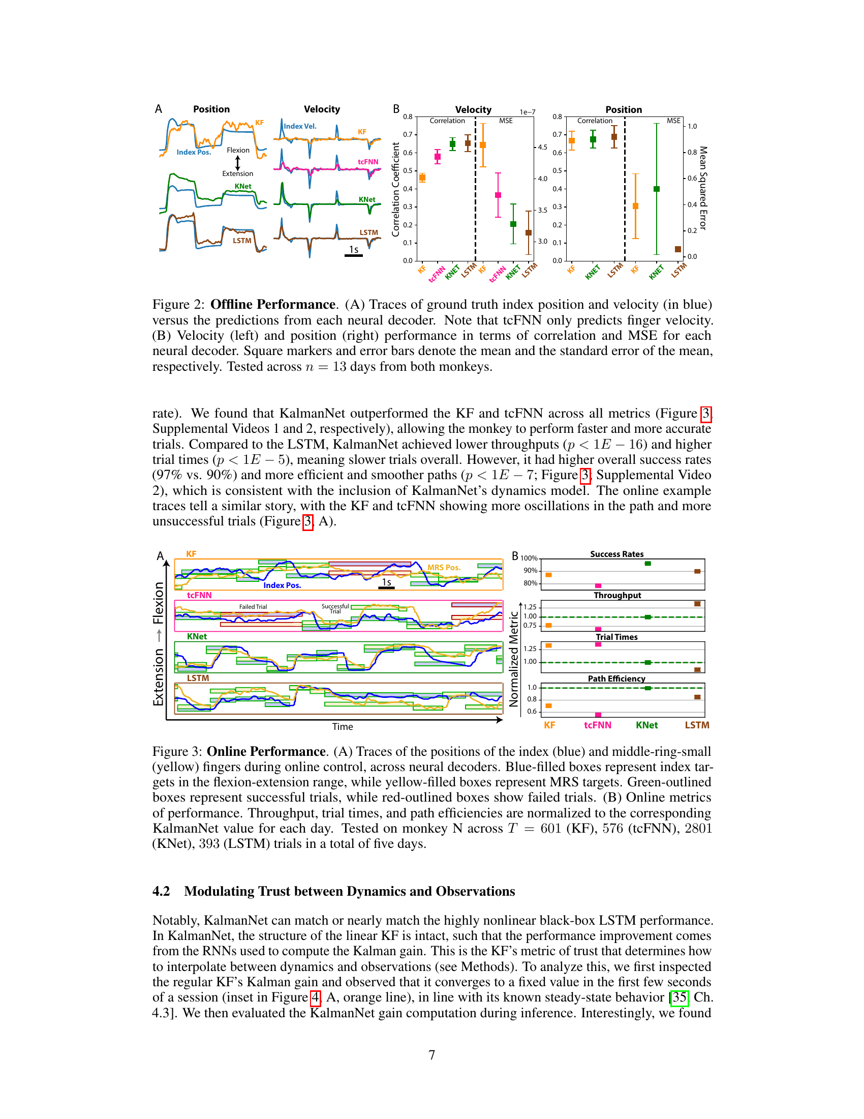
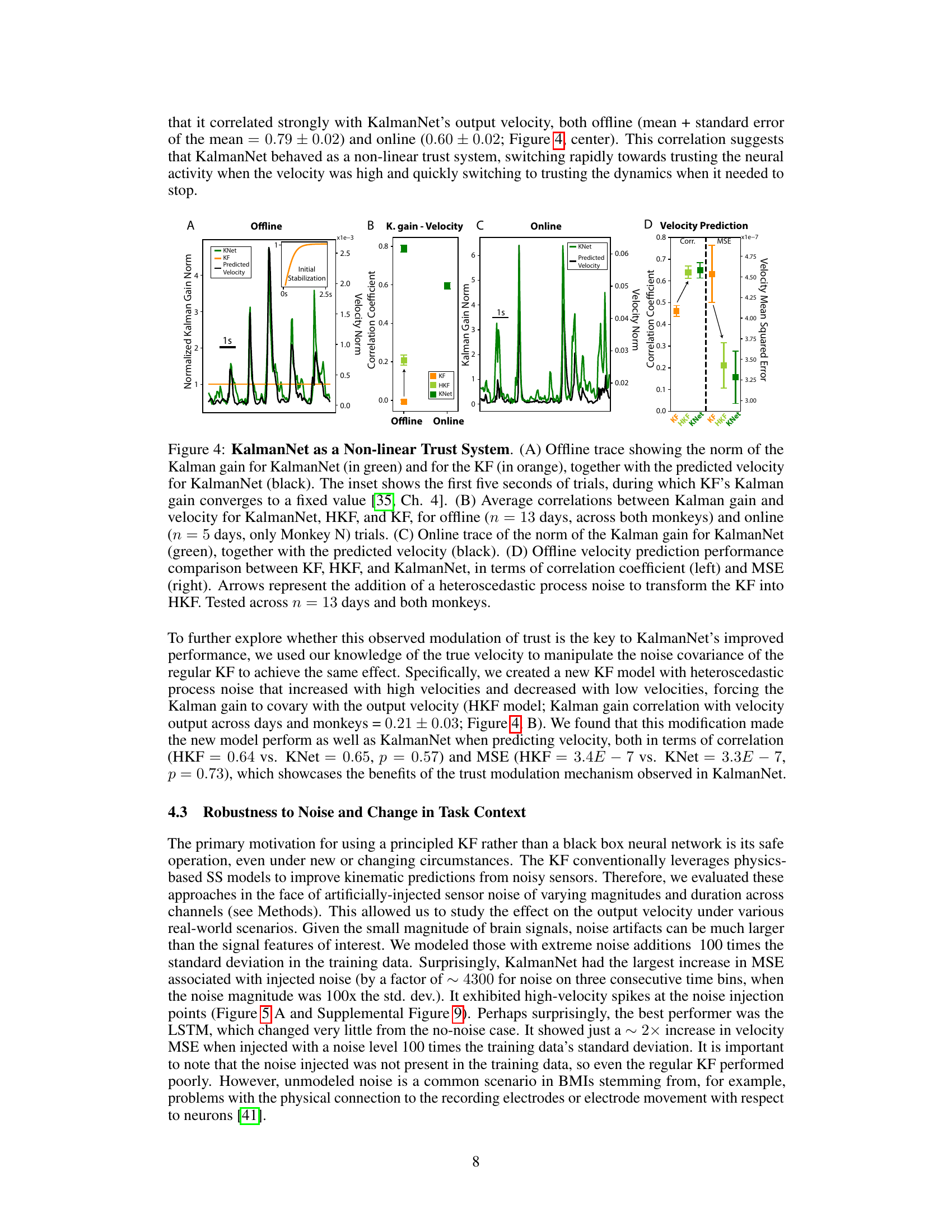
Offline evaluations of the deep learning models, including KalmanNet, revealed comparable performance to state-of-the-art methods in predicting finger kinematics from neural data. KalmanNet demonstrated statistically significant improvements over the Kalman filter, particularly in terms of correlation and MSE in velocity predictions. The online experiments showed that KalmanNet enabled monkeys to complete trials more accurately and efficiently than simpler models, achieving higher success rates and smoother paths, while the LSTM showed faster trials. However, KalmanNet’s performance gains did not always translate into faster information throughput compared to the LSTM. A key finding is KalmanNet’s ability to modulate its trust between dynamical models and direct neural inputs, demonstrated by a strong correlation between its Kalman gain and the predicted velocity. This flexible trust mechanism may explain why the model excels in some aspects, while showing limitations in others, such as generalization.
Noise Robustness#
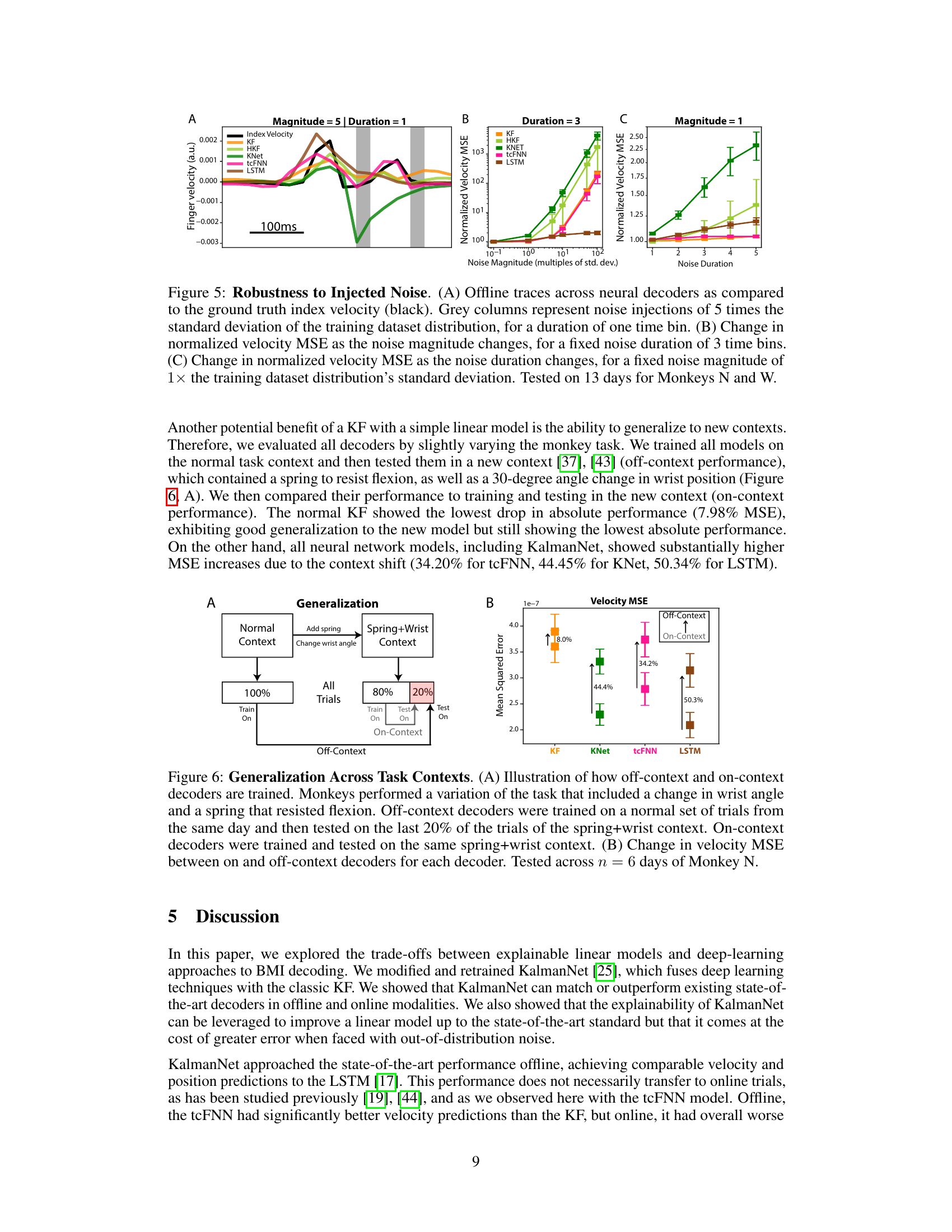
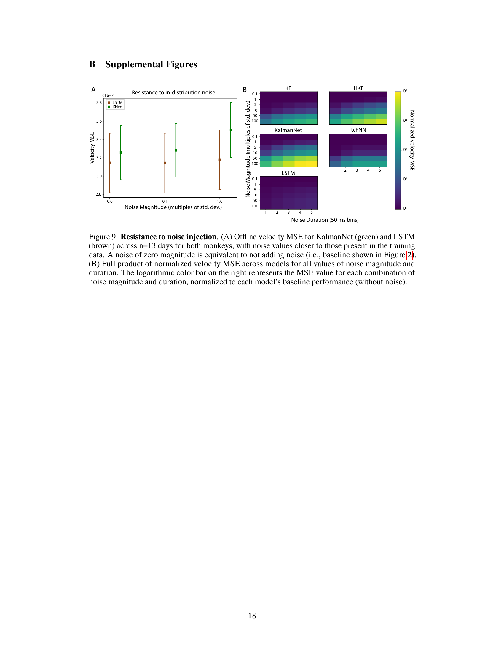
The research explores the robustness of various brain-machine interface (BMI) decoders to noise. KalmanNet, surprisingly, showed the lowest robustness to high-magnitude, out-of-distribution noise, exhibiting large velocity spikes in response. This contrasts with the LSTM, which demonstrated significantly higher noise resilience, experiencing only a twofold increase in MSE even under extreme noise conditions. This result challenges conventional assumptions about the safety and reliability of model-based approaches like Kalman filters in noisy environments, highlighting the unexpected strengths of purely data-driven models like LSTMs. The findings emphasize the critical need for rigorous noise testing across diverse BMI decoder architectures to ensure real-world performance and safety. Further investigation into the specific mechanisms behind KalmanNet’s sensitivity to noise is essential, possibly involving exploring outlier-robust Kalman filter variations or incorporating hypernetworks to handle varying noise levels more effectively.
Generalization Limits#
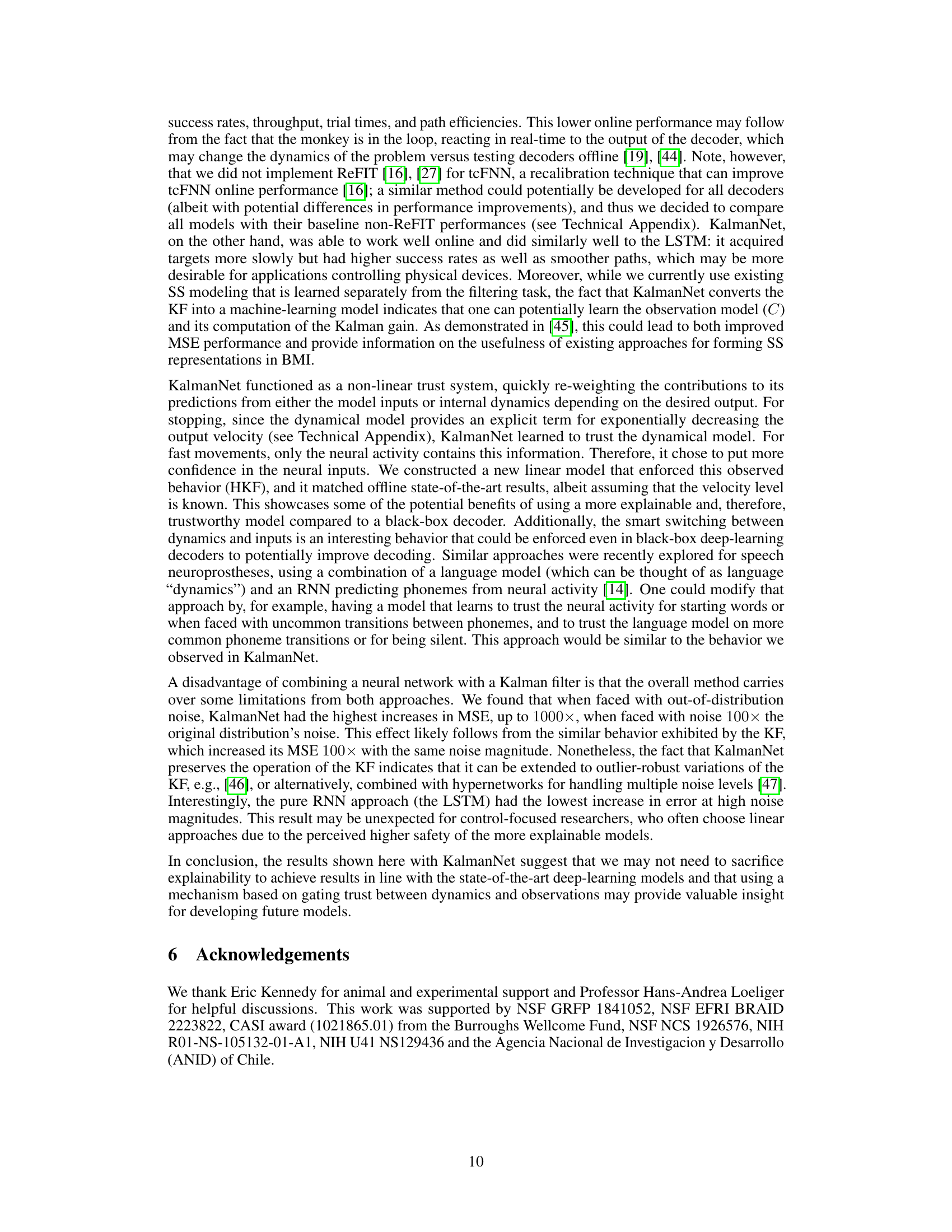
The concept of ‘Generalization Limits’ in the context of brain-machine interfaces (BMIs) using deep learning models is critical. Deep learning models, while achieving high performance on specific tasks and datasets, often struggle to generalize to unseen data or different contexts. This limitation stems from their reliance on learning intricate patterns within the training data, potentially including noise or task-specific artifacts, rather than robust underlying principles. For BMIs, poor generalization can manifest as unpredictable or unsafe behavior when a trained decoder encounters a new situation (e.g., different neural activity patterns, altered environmental conditions). Therefore, understanding and mitigating these limits is paramount for reliable BMI applications. Explainable models, in contrast, often show better generalization because their simpler structure and reliance on established principles result in less overfitting to specific training data. However, explainable models may sacrifice some performance compared to deep learning models. The challenge lies in finding a balance: enhancing generalization capacity without sacrificing the performance or explainability that are desired in BMIs.
More visual insights#
More on figures

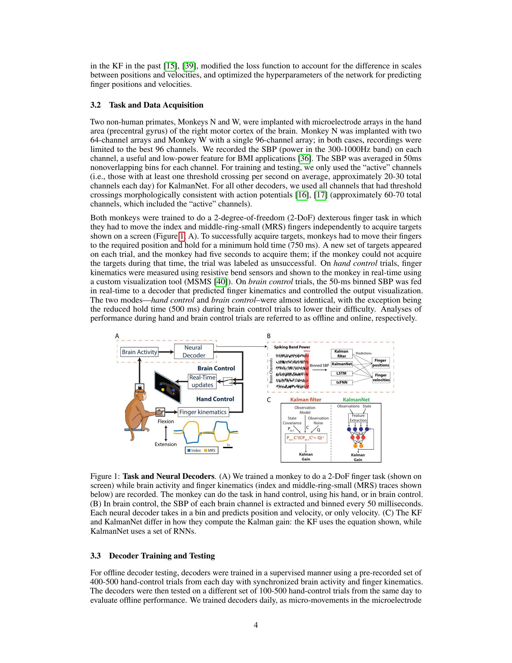
🔼 This figure displays the offline performance comparison of four neural decoders (KF, tcFNN, KalmanNet, and LSTM) in predicting finger kinematics from brain data. Panel (A) shows example traces of ground truth and predicted finger positions and velocities, highlighting the performance differences between the decoders. Panel (B) provides a quantitative comparison using correlation coefficients and mean squared errors (MSE) for both velocity and position predictions, calculated over 13 days of data from two monkeys. Error bars represent the standard error of the mean.
read the caption
Figure 2: Offline Performance. (A) Traces of ground truth index position and velocity (in blue) versus the predictions from each neural decoder. Note that tcFNN only predicts finger velocity. (B) Velocity (left) and position (right) performance in terms of correlation and MSE for each neural decoder. Square markers and error bars denote the mean and the standard error of the mean, respectively. Tested across n = 13 days from both monkeys.

🔼 This figure shows a comparison of the online performance of four different neural decoders (KF, tcFNN, KalmanNet, and LSTM) for controlling finger movements in a monkey. Panel A displays time series data showing the index and middle-ring-small finger positions for successful and failed trials for each decoder. Panel B presents a bar graph summarizing the performance metrics (success rate, throughput, trial times, and path efficiency) for each decoder, normalized to KalmanNet’s performance for easier comparison. The results show that KalmanNet outperforms other decoders in most metrics.
read the caption
Figure 3: Online Performance. (A) Traces of the positions of the index (blue) and middle-ring-small (yellow) fingers during online control, across neural decoders. Blue-filled boxes represent index targets in the flexion-extension range, while yellow-filled boxes represent MRS targets. Green-outlined boxes represent successful trials, while red-outlined boxes show failed trials. (B) Online metrics of performance. Throughput, trial times, and path efficiencies are normalized to the corresponding KalmanNet value for each day. Tested on monkey N across T = 601 (KF), 576 (tcFNN), 2801 (KNet), 393 (LSTM) trials in a total of five days.
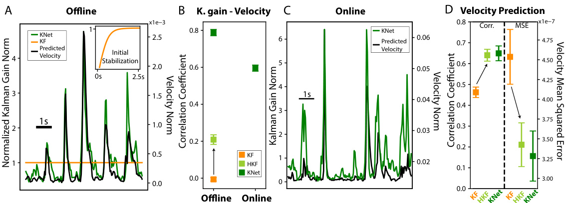
🔼 This figure demonstrates KalmanNet’s ability to modulate its trust between the dynamics model and neural observations, acting as a non-linear trust system. Panel A shows an offline trace comparing KalmanNet’s Kalman gain (a measure of trust) with the KF’s Kalman gain and predicted velocity. Panel B presents the average correlation between Kalman gain and velocity for KalmanNet, HKF (heteroscedastic Kalman filter), and KF, across both offline and online trials. Panel C displays an online trace mirroring panel A’s analysis. Finally, panel D offers a comparison of offline velocity prediction performance (correlation and MSE) between KF, HKF, and KalmanNet, highlighting the performance boost achieved by modulating trust using a recurrent neural network.
read the caption
Figure 4: KalmanNet as a Non-linear Trust System. (A) Offline trace showing the norm of the Kalman gain for KalmanNet (in green) and for the KF (in orange), together with the predicted velocity for KalmanNet (black). The inset shows the first five seconds of trials, during which KF’s Kalman gain converges to a fixed value [35, Ch. 4]. (B) Average correlations between Kalman gain and velocity for KalmanNet, HKF, and KF, for offline (n = 13 days, across both monkeys) and online (n = 5 days, only Monkey N) trials. (C) Online trace of the norm of the Kalman gain for KalmanNet (green), together with the predicted velocity (black). (D) Offline velocity prediction performance comparison between KF, HKF, and KalmanNet, in terms of correlation coefficient (left) and MSE (right). Arrows represent the addition of a heteroscedastic process noise to transform the KF into HKF. Tested across n = 13 days and both monkeys.

🔼 This figure demonstrates how different neural decoders respond to injected noise in offline settings. Panel A shows example velocity traces for each decoder with a noise injection. Panels B and C illustrate how mean squared error (MSE) changes as a function of noise magnitude (B) and duration (C). The results reveal that KalmanNet is most sensitive to the injected noise, while LSTM is most robust.
read the caption
Figure 5: Robustness to Injected Noise. (A) Offline traces across neural decoders as compared to the ground truth index velocity (black). Grey columns represent noise injections of 5 times the standard deviation of the training dataset distribution, for a duration of one time bin. (B) Change in normalized velocity MSE as the noise magnitude changes, for a fixed noise duration of 3 time bins. (C) Change in normalized velocity MSE as the noise duration changes, for a fixed noise magnitude of 1x the training dataset distribution’s standard deviation. Tested on 13 days for Monkeys N and W.

🔼 This figure demonstrates the generalization ability of different decoders across varying task contexts. Panel A illustrates the training and testing procedures for both off-context (trained on normal tasks, tested on a spring-restrained task) and on-context (trained and tested on the spring-restrained task) decoders. Panel B presents the results, showing the increase in mean squared error (MSE) for velocity predictions when decoders are tested in an unfamiliar task context (off-context). The Kalman filter demonstrates superior generalization compared to the deep-learning models (KalmanNet, tcFNN, and LSTM).
read the caption
Figure 6: Generalization Across Task Contexts. (A) Illustration of how off-context and on-context decoders are trained. Monkeys performed a variation of the task that included a change in wrist angle and a spring that resisted flexion. Off-context decoders were trained on a normal set of trials from the same day and then tested on the last 20% of the trials of the spring+wrist context. On-context decoders were trained and tested on the same spring+wrist context. (B) Change in velocity MSE between on and off-context decoders for each decoder. Tested across n = 6 days of Monkey N.
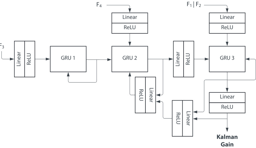
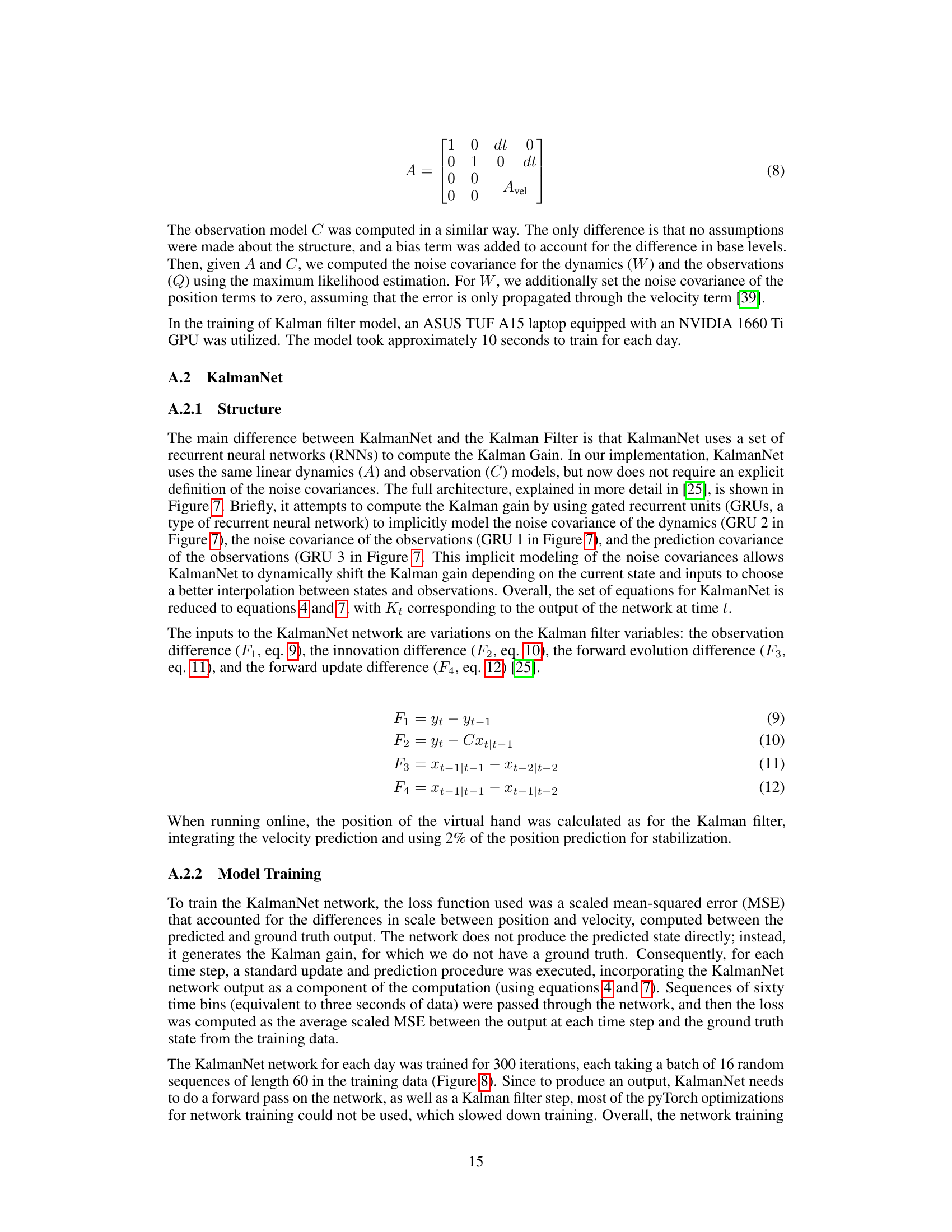
🔼 This figure shows the architecture of the KalmanNet model. KalmanNet uses a recurrent neural network (RNN) to calculate the Kalman gain, which determines the balance between dynamical predictions and observations. The inputs to the network are four feature vectors (F1, F2, F3, F4) representing differences between current and past Kalman filter states and observations. These features are processed through three gated recurrent units (GRUs) and several linear layers with ReLU activation functions. The output of the network is the Kalman gain, which is used to update the state estimate.
read the caption
Figure 7: KalmanNet architecture. Diagram of the components of the KalmanNet network. It consists of three GRUs plus seven linear + ReLU layers that try to model the normal way of computing the Kalman gain [25]. F1 through F4 correspond to the input features from equations 9 through 12.
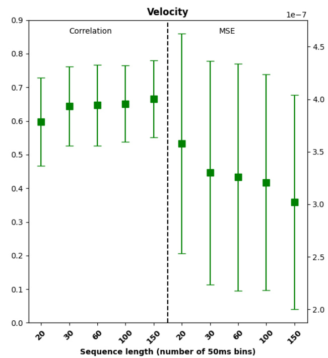
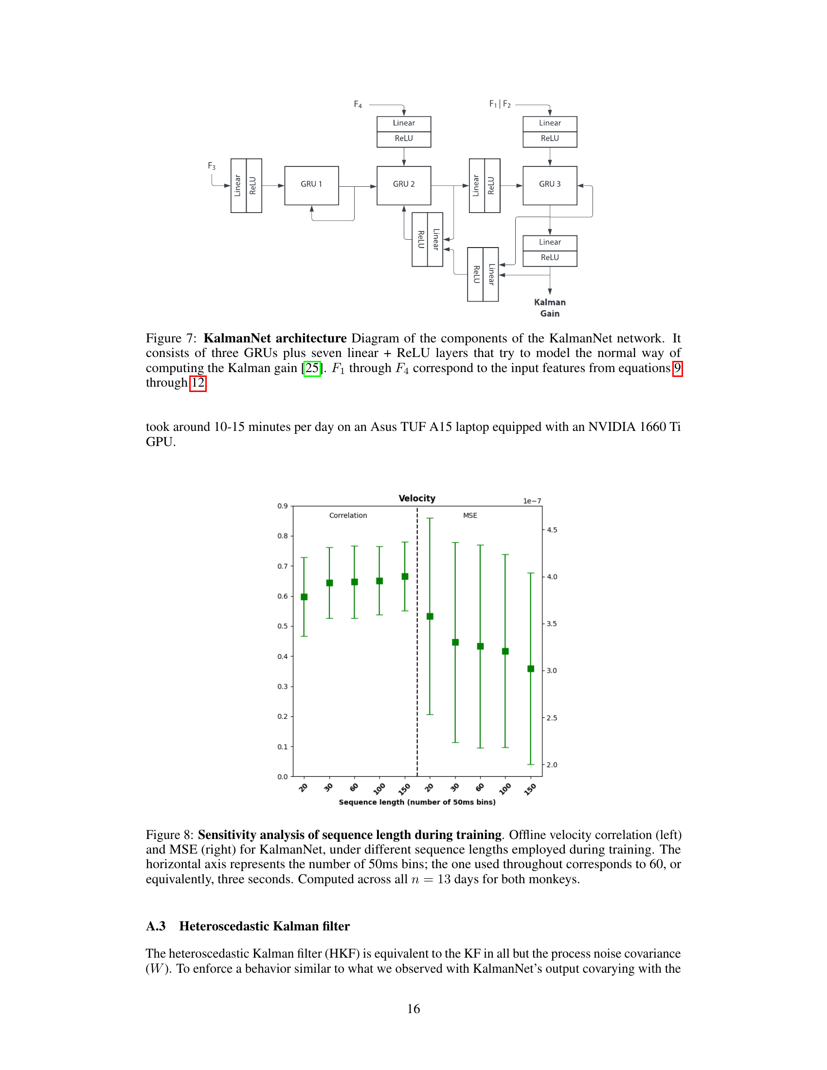
🔼 This figure displays the results of a sensitivity analysis performed to determine the optimal sequence length used for training the KalmanNet model. The analysis compares the model’s performance across different sequence lengths in terms of velocity correlation and mean squared error (MSE). The results are shown as error bars, indicating the variability across 13 days of testing with two monkeys. The optimal sequence length was found to be 60 bins (3 seconds).
read the caption
Figure 8: Sensitivity analysis of sequence length during training. Offline velocity correlation (left) and MSE (right) for KalmanNet, under different sequence lengths employed during training. The horizontal axis represents the number of 50ms bins; the one used throughout corresponds to 60, or equivalently, three seconds. Computed across all n = 13 days for both monkeys.
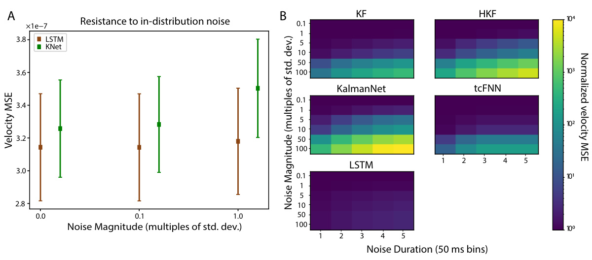
🔼 Figure 9 shows the results of evaluating the robustness of KalmanNet and other models to noise in real-world scenarios. (A) shows a comparison of the mean squared error (MSE) for KalmanNet and LSTM at varying noise magnitudes, showing that LSTM is more resistant to out-of-distribution noise. (B) presents a heatmap summarizing the MSE across all models tested for combinations of noise magnitude and duration, highlighting the sensitivity of each model to these types of noise.
read the caption
Figure 9: Resistance to noise injection. (A) Offline velocity MSE for KalmanNet (green) and LSTM (brown) across n=13 days for both monkeys, with noise values closer to those present in the training data. A noise of zero magnitude is equivalent to not adding noise (i.e., baseline shown in Figure 2). (B) Full product of normalized velocity MSE across models for all values of noise magnitude and duration. The logarithmic color bar on the right represents the MSE value for each combination of noise magnitude and duration, normalized to each model’s baseline performance (without noise).
Full paper#

