↗ OpenReview ↗ NeurIPS Homepage ↗ Chat
TL;DR#
Traditional outlier removal methods often employ a two-stage process: outlier detection followed by estimation on the cleaned data. This approach can be suboptimal as outlier removal isn’t informed by the estimation task itself. This leads to potential inefficiencies and inaccuracies, particularly when dealing with complex datasets or intricate models.
This paper tackles these issues by proposing a novel single-step outlier rectification method. The core idea involves using optimal transport with a concave cost function to identify and rectify outliers while simultaneously performing the estimation task. This joint optimization approach ensures that outlier removal directly benefits the estimation process, resulting in more accurate and robust results. The effectiveness of the method is demonstrated through simulations and real-world applications, showcasing significant improvements over conventional approaches.
Key Takeaways#
Why does it matter?#
This paper is crucial for researchers working on robust statistics and machine learning. It introduces a novel framework for outlier detection and rectification, significantly improving the accuracy and reliability of estimations in various applications. The integration of outlier rectification and estimation within a single optimization process is a major advancement, addressing the limitations of traditional two-stage methods. This work opens up new avenues for research in developing more robust and efficient estimators for a wide range of statistical and machine learning problems.
Visual Insights#

This figure illustrates the data-driven decision-making cycle, highlighting the three main stages: data generation, model building, and out-of-sample environment. It emphasizes that the data-generating distribution may be contaminated (P’), leading to a data-driven model (P’n) that may perform poorly in the true out-of-sample environment (P~). The arrows show the flow of information from the contaminated data to model building and ultimately, to the out-of-sample performance.

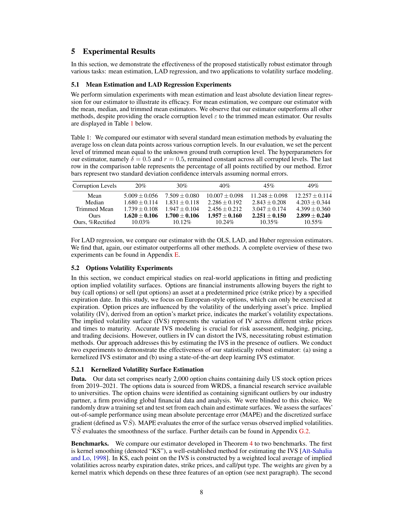
This table compares the performance of the proposed statistically robust estimator against several standard mean estimation methods (mean, median, trimmed mean). The comparison is based on the average loss calculated on clean data points for different corruption levels (20%, 30%, 40%, 45%). The hyperparameters of the proposed estimator (δ and r) are kept constant across all corruption levels. The last row shows the percentage of points rectified by the proposed method for each corruption level. Error bars represent 95% confidence intervals, assuming data is normally distributed.
In-depth insights#
Optimal Transport#
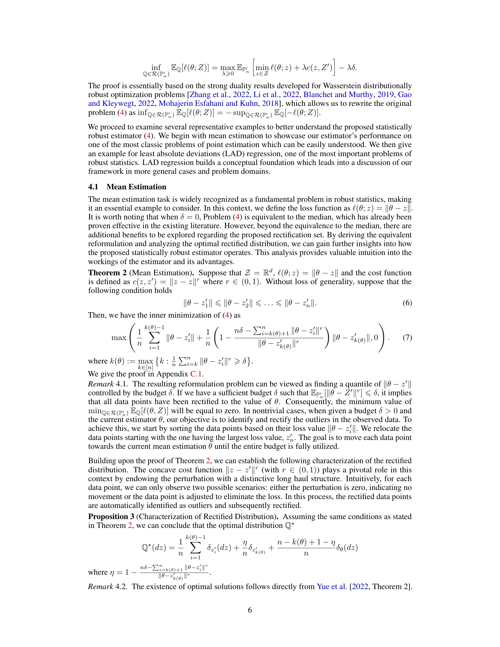
The concept of Optimal Transport (OT) is central to the research paper’s novel approach for outlier rectification. OT provides a framework for measuring the distance between probability distributions, moving beyond traditional distance metrics. The authors leverage a concave cost function within the OT framework, a key innovation that incentivizes the movement of outliers towards the bulk of the data, effectively rectifying them. This contrasts with typical convex cost functions used in OT, which might distribute adjustments evenly between the data points. The integration of OT with estimation in a joint optimization framework is a major contribution, creating a unified process. This addresses limitations of two-stage methods that often separate outlier detection and estimation, which can lead to suboptimal results. The choice of a concave cost function in OT is crucial to the algorithm’s ability to identify and rectify outliers effectively during the optimization process. The authors’ method demonstrates significant improvements over traditional approaches in simulation and real-world applications, highlighting the power and flexibility of OT in robust statistical estimation.
Concave Cost#
The concept of a “concave cost” function within the context of optimal transport is crucial for the effectiveness of the proposed outlier rectification mechanism. Unlike convex cost functions, which encourage short, local movements of data points, a concave cost function incentivizes “long haul” transport. This means that outliers, which are far from the bulk of the data, are more readily moved significant distances towards the central tendency, effectively rectifying them. This characteristic is key to automatically identifying and correcting outliers during the optimization process. The concave cost function is demonstrably more effective than convex counterparts at achieving accurate model estimation in the presence of outliers, as shown in the simulations and real-world applications presented. The choice of concave cost function is not arbitrary, but rather a deliberate design choice aimed at achieving robust statistical estimation in the presence of contamination, thereby improving the overall quality and reliability of model results. The selection of the cost function’s specific parameters, however, requires careful consideration and is demonstrated to have a significant impact on model performance.
Outlier Rectification#
The concept of ‘Outlier Rectification’ in the context of this research paper centers on integrating outlier detection and data estimation within a unified optimization framework. Traditional methods often involve a two-step process—detecting and removing outliers, then estimating parameters using the cleaned data. This approach is suboptimal because outlier removal isn’t informed by the estimation task, potentially leading to inefficient parameter estimates. The proposed method addresses this limitation by using optimal transport with a concave cost function to define a rectification set. This set contains probability distributions close to the original, contaminated distribution, while implicitly penalizing outliers through the choice of cost function. The optimal distribution within the rectification set is then used for parameter estimation, thus effectively integrating both outlier rectification and the estimation task into a single optimization process. The concave cost function is critical, enabling the algorithm to move outliers toward the data’s central tendency rather than simply shifting all points closer to each other, which is the pitfall of the convex cost function. This approach is demonstrated to be more effective than conventional methods for mean estimation, least absolute regression, and option implied volatility surface fitting.
Robust Estimation#
Robust estimation focuses on developing statistical methods that are resilient to outliers and data contamination. Traditional methods often break down in the presence of such anomalies. Robust approaches aim to minimize the influence of outliers on parameter estimates, enhancing the reliability and accuracy of results. M-estimators and minimum distance functionals represent established techniques. Optimal transport methods provide a novel framework where outlier rectification and estimation are integrated, addressing the limitations of two-stage procedures. Concave cost functions within optimal transport are key to effectively identifying and correcting outliers, offering a significant advantage over traditional techniques. Simulations and empirical results across various statistical applications validate the improved robustness and efficiency of these new approaches.
IVS Applications#
Implied Volatility Surface (IVS) applications are of significant interest in finance, particularly in option pricing and risk management. Accurate IVS modeling is crucial for correctly pricing options, as inaccuracies can lead to substantial financial losses. This is particularly important for complex products whose prices are directly derived from the IVS. Robust IVS estimation techniques are essential to mitigate the impact of outliers and noisy data, which can significantly distort the surface and affect model accuracy. The use of robust statistical methods, particularly those that integrate outlier rectification and estimation in a unified framework, is critical to improve accuracy and reliability of IVS models. Concave cost functions in optimal transport show promise in automatically identifying and correcting outliers, leading to smoother and more accurate surfaces. Empirical testing on real market data is critical to validate the effectiveness of any new IVS estimation approach, comparing performance metrics like Mean Average Percentage Error (MAPE) and surface smoothness against established benchmarks.
More visual insights#
More on figures

This figure shows how the proposed estimator rectifies outlier data points using a concave cost function in the optimal transport framework. It presents three scenarios with varying budget parameters (δ): δ=0, δ=0.9, and δ=1.5. Each scenario displays the original data (clean data points in blue and outlier data points in orange), the rectified data points (in green), the true underlying distribution (black line), and the rectified distribution estimated by the proposed estimator (red line). The concave cost function’s effectiveness in pulling outlier data points towards the main distribution is visually illustrated, showcasing the improvement in estimation accuracy as the budget increases.

This figure shows how the proposed estimator rectifies data points with a concave cost function (r=0.5) under different budget values (δ). It compares the results across three different budgets: δ = 0, δ = 0.9, and δ = 1.5. For each budget level, the figure displays the original clean and outlier data points, the rectified outlier data points, the ground truth line, and the line of best fit produced by the estimator. The visualization demonstrates how the concave cost function effectively moves outlier points closer to the bulk of the clean data distribution, resulting in improved performance. This illustrates the efficacy of the concave cost function in correctly rectifying outliers compared to the convex case, which leads to incorrect fits as shown in the next figure.
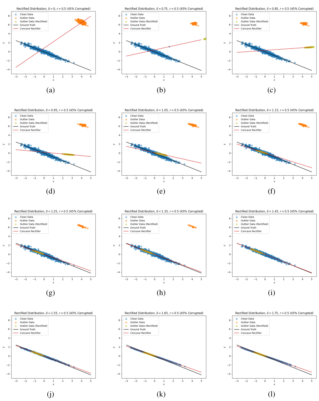
This figure shows the results of applying the proposed outlier rectification method with a concave cost function (r = 0.5) to simulated data with different budget parameters (δ). Each subfigure presents the original data (clean and outlier data), the rectified data (outlier data is rectified), the ground truth line of best fit, and the estimated line of best fit using the proposed method. The results illustrate how the concave cost function effectively rectifies outliers and the effect of the budget parameter on the results.

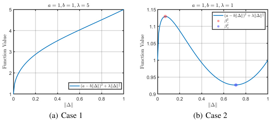
The figure shows a plot of an irregular objective function, highlighting the challenges in solving optimization problems with such functions. The presence of downward-facing cusps in the graph indicates a lack of subdifferential regularity, making it difficult to compute first-order oracles necessary for optimization algorithms.

The figure visualizes the results of a mean estimation experiment. Subfigure (a) shows the original data distribution with outliers. Subfigure (b) presents the rectified data distribution after applying the proposed outlier rectification method with δ=2.5, demonstrating the successful identification and movement of outliers toward the mean. Subfigure (c) displays a sensitivity analysis showing the effect of different δ values on the mean loss, indicating relative insensitivity and graceful degradation towards the median estimator at extreme values of δ.

This figure shows the results of LAD regression on data with outliers. (a) shows the fitted lines for different methods (OLS, LAD, Huber, and the proposed method) on the original data. (b) and (c) show the rectified data (outliers moved) and the fitted line for the proposed method using different budget parameters (δ = 1 and δ = 1.5). The proposed method effectively rectifies the outliers, leading to a better fit.

This figure visualizes the results of LAD regression experiments. Subfigure (a) compares the lines of best fit produced by various methods (OLS, LAD, Huber, and the proposed method) on a dataset with 45% outliers. Subfigures (b) and (c) show how the proposed method rectifies outliers with different budget parameters (d = 1 and d = 1.5, respectively). The visualization demonstrates how the proposed method outperforms other methods, especially with larger budgets, achieving a line of best fit closer to the true line.
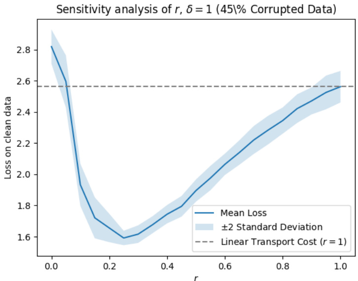
The figure visualizes the performance of the proposed statistically robust estimator on mean estimation tasks. Panel (a) shows the original data with outliers. Panel (b) displays the rectified data after applying the proposed method with a budget parameter δ = 2.5. Panel (c) presents a sensitivity analysis illustrating the impact of various δ values on the estimation performance, demonstrating robustness and graceful degradation to the median estimator in extreme cases.
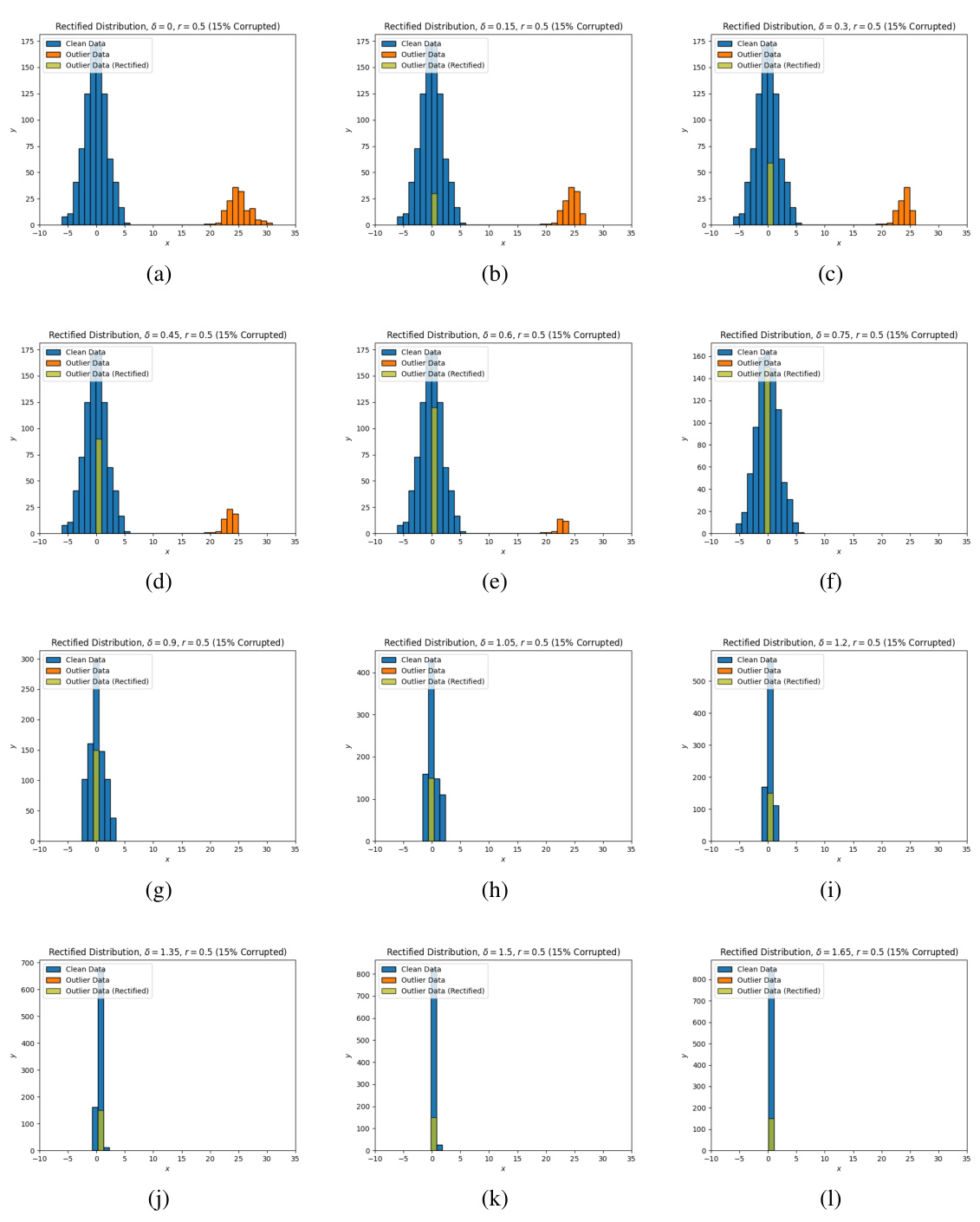
This figure shows the evolution of the rectified distribution produced by the estimator under various values of delta (δ) for the concave cost function with r = 0.5. Each subplot represents a different delta value, showing how the distribution of clean data (blue) and outliers (orange) changes as delta is increased. The rectified distribution (green) illustrates the effect of the proposed method in mitigating outliers by moving them towards the clean data distribution.
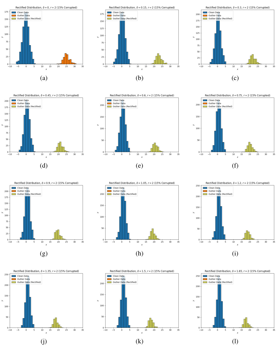
This figure visualizes how the rectified distribution evolves with different budget parameters (δ) for a concave cost function (r = 0.5). Each subplot shows a histogram representing the distribution of data points after rectification, highlighting how outliers are moved closer to the main data cluster as the budget increases. It demonstrates the impact of the concave cost function on outlier rectification, showcasing the effectiveness of the proposed method in adjusting the distribution to improve the accuracy of estimation.
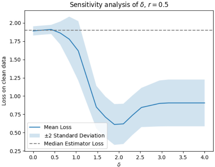
This figure visualizes the effect of the proposed outlier rectification mechanism. Subfigure (a) shows the original data distribution with outliers. Subfigure (b) displays how the proposed method rectifies the outliers, moving them closer to the true distribution. Subfigure (c) shows the sensitivity analysis of the budget parameter (δ), demonstrating that the method’s performance remains robust across a wide range of δ values.
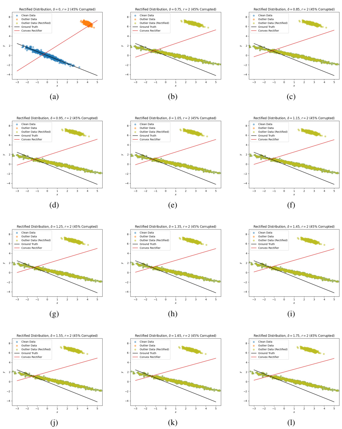
This figure compares the results of using a convex cost function in the optimal transport-based rectification set, with the concave cost function results shown in Figure 2. The plots show the original clean data (blue), outlier data (orange), the rectified data (green), the ground truth line of best fit (black dashed line), and the line of best fit produced by the estimator (red). For the convex cost function, regardless of the budget (δ = 0, 0.9, 1.5), all data points are rectified towards each other. This shows that the convex cost is not effective for our purposes, in contrast to the concave cost shown in Figure 2.
This figure shows how the proposed estimator rectifies the data with a concave cost function (r=0.5) for different budget values (δ). The top row displays the results for budgets of δ = 0, δ = 0.9, and δ = 1.5, respectively. Each plot shows the clean data (blue), the outlier data (orange), the rectified outlier data (green), the ground truth line, and the line fit by the estimator (red). The key observation is that the concave cost function effectively moves outlier points towards the main cluster. As δ increases, more outliers are moved, leading to a better fit with the ground truth.
This figure shows the results of using the proposed estimator with a concave cost function (r=0.5) on simulated data with 45% corruption. It compares the rectified data (green) with the original data (blue and orange outliers). The results are shown for different values of the budget parameter (δ = 0, 0.9, 1.5), illustrating how increasing the budget improves outlier rectification. The ground truth (black line) and the estimator’s fit (red line) are also shown, demonstrating the impact of outlier rectification on model accuracy.

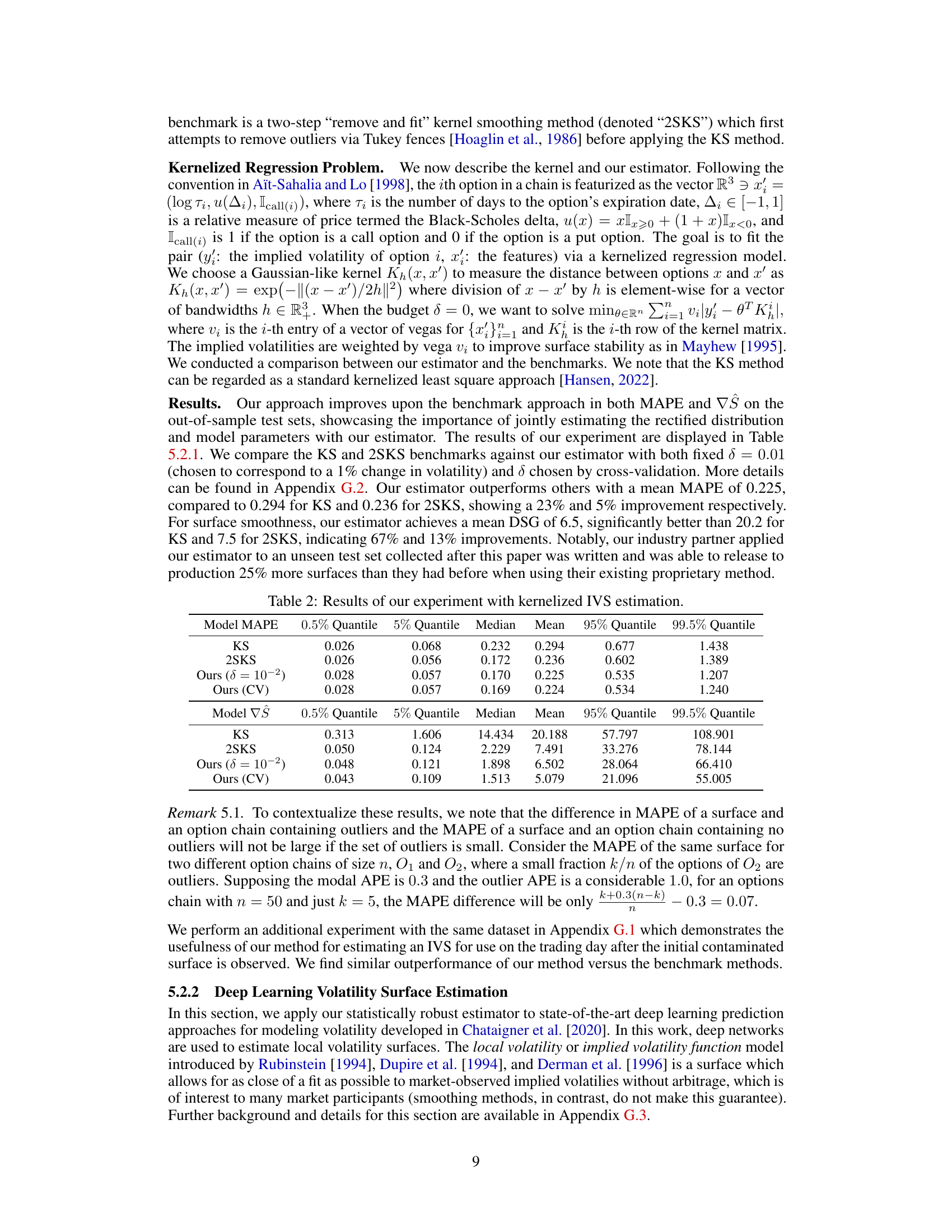
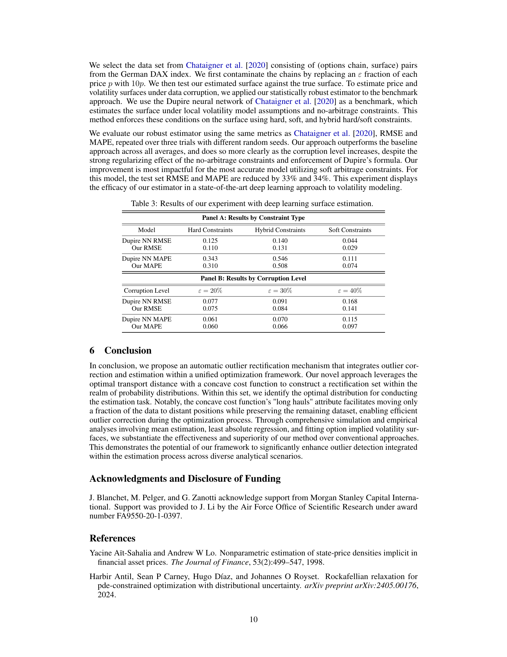
This figure shows the option implied volatility surface estimated using the benchmark KS method. The plot highlights outliers in the data, which significantly affect the accuracy of the surface estimation, resulting in unrealistic volatility values and a steep surface gradient.

This figure shows the implied volatility surface estimated using the kernel smoothing (KS) benchmark method. The surface is heavily distorted by outliers present in the data (shown as blue and red dots). These outliers significantly impact the accuracy and smoothness of the surface.
More on tables

This table compares the performance of the proposed statistically robust estimator with several standard mean estimation methods (mean, median, trimmed mean) across different corruption levels (20%, 30%, 40%, 45%, 49%). The average loss on clean data points is evaluated for each method. The hyperparameters of the proposed estimator are kept constant. The last row shows the percentage of points rectified by the proposed method. Error bars indicate two standard deviations.

This table compares the performance of the proposed statistically robust estimator against several standard mean estimation methods (mean, median, trimmed mean) across various levels of data corruption. The performance is measured by average loss on clean data points. The hyperparameters of the proposed estimator are kept constant, while the trimmed mean’s percentage is set to match the true corruption level. The last row shows the percentage of data points rectified by the new method.
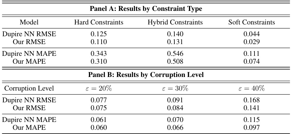
This table compares the performance of the proposed statistically robust estimator against several standard mean estimation methods (mean, median, trimmed mean) across different corruption levels. The performance is measured by the average loss on clean data points. The hyperparameters for the proposed estimator were kept constant across all corruption levels. The table also shows the percentage of data points rectified by the method for each corruption level.

This table compares the performance of the proposed statistically robust estimator against several standard mean estimation methods (mean, median, trimmed mean) across different corruption levels (20%, 30%, 40%, 45%, 49%). The average loss on clean data points is used as the evaluation metric. The hyperparameters of the proposed estimator (δ and r) are kept constant. The last row indicates the percentage of data points rectified by the method.

This table compares the performance of the proposed statistically robust estimator against several standard mean estimation methods (mean, median, trimmed mean) across different corruption levels (20%, 30%, 40%, 45%). The hyperparameters of the proposed estimator are kept constant. The results show the average loss on clean data points and the percentage of points rectified by the estimator at each corruption level. Error bars indicate two standard deviations.
Full paper#
