TL;DR#
Imputation of missing values in multivariate time series is crucial for many applications, but existing methods struggle with accuracy, particularly concerning the residual term. This is because the residual term is the most challenging component to model, as it represents the complex and variable parts of the data. Inaccurate residual imputation leads to overall lower accuracy in time series analysis.
The researchers propose a novel method, Frequency-aware Generative Models for Multivariate Time Series Imputation (FGTI), to address these limitations. FGTI uses a high-frequency filter to improve imputation of the residual term, combining this with deep representation learning techniques. Results show FGTI outperforms existing methods in several real-world datasets, demonstrating its efficacy in improving both imputation accuracy and downstream application performance. This is a significant advancement in the field.
Key Takeaways#
Why does it matter?#
This paper is important because it addresses a critical issue in time series analysis: accurate imputation of missing data. The proposed Frequency-aware Generative Model (FGTI) offers a novel approach that outperforms existing methods, particularly in handling the complex residual term. This opens new avenues for research in this crucial area and could significantly improve the performance of downstream applications reliant on multivariate time series data. Its focus on high-frequency components of residual data is a unique contribution that enhances imputation accuracy and holds significant implications for various applications.
Visual Insights#
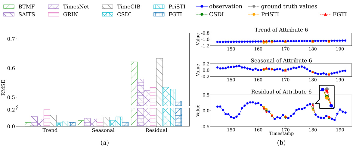
🔼 The figure shows a bar chart comparing the imputation accuracy of different methods (BTMF, SAITS, TimesNet, GRIN, TimeCIB, CSDI, PriSTI, FGTI) for three components of multivariate time series data: trend, seasonal, and residual. The residual component shows significantly higher error than trend and seasonal components for all methods, highlighting the importance of accurately imputing the residual term for better overall imputation performance. A secondary plot shows a line graph with zoomed-in views of trend, seasonal, and residual components of a specific attribute (Attribute 6) from the KDD dataset, further illustrating the relatively higher error associated with the residual term imputation.
read the caption
Figure 1: Improving the imputation accuracy of the residual term is the key to boosting the imputation performance of the model.
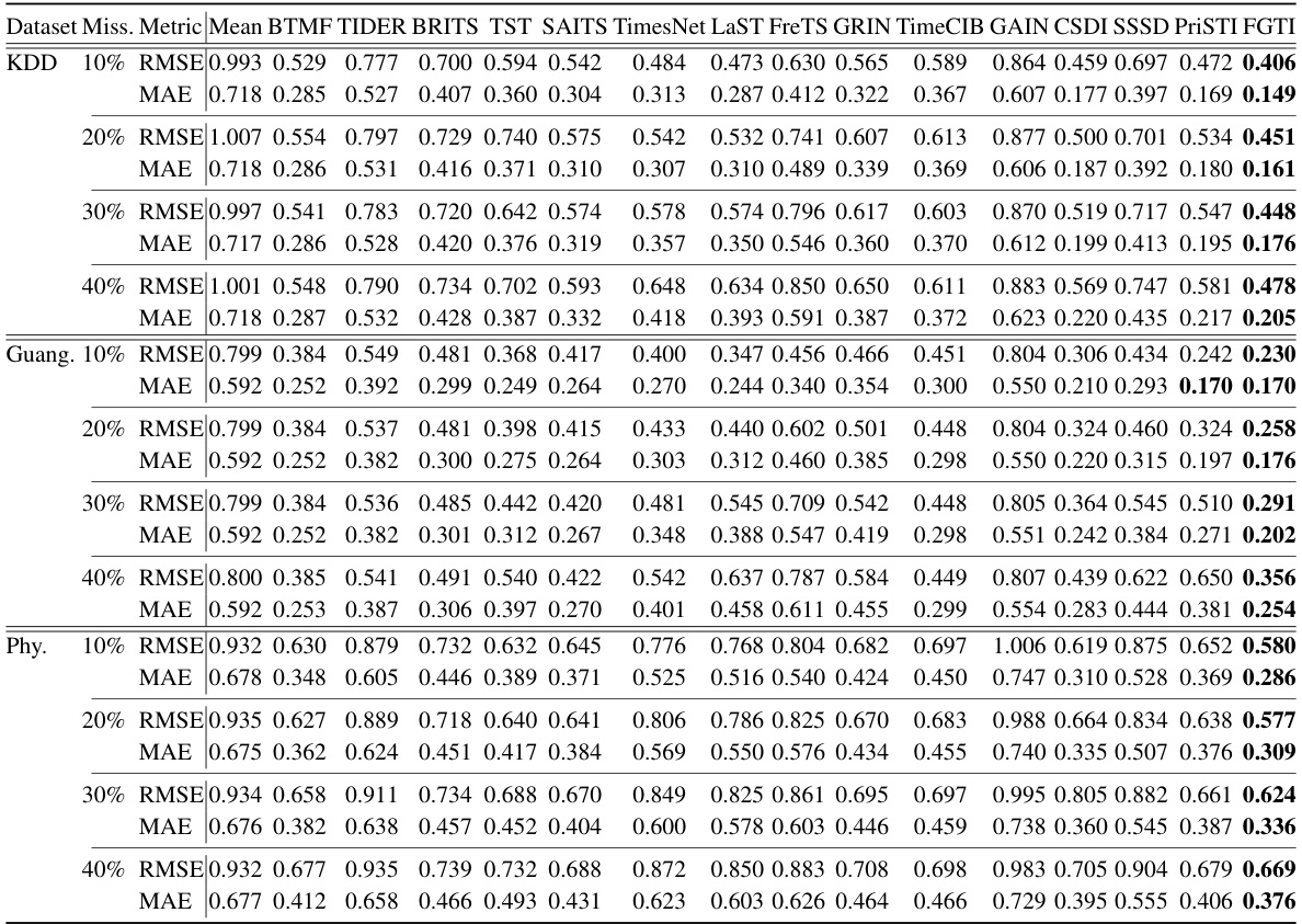
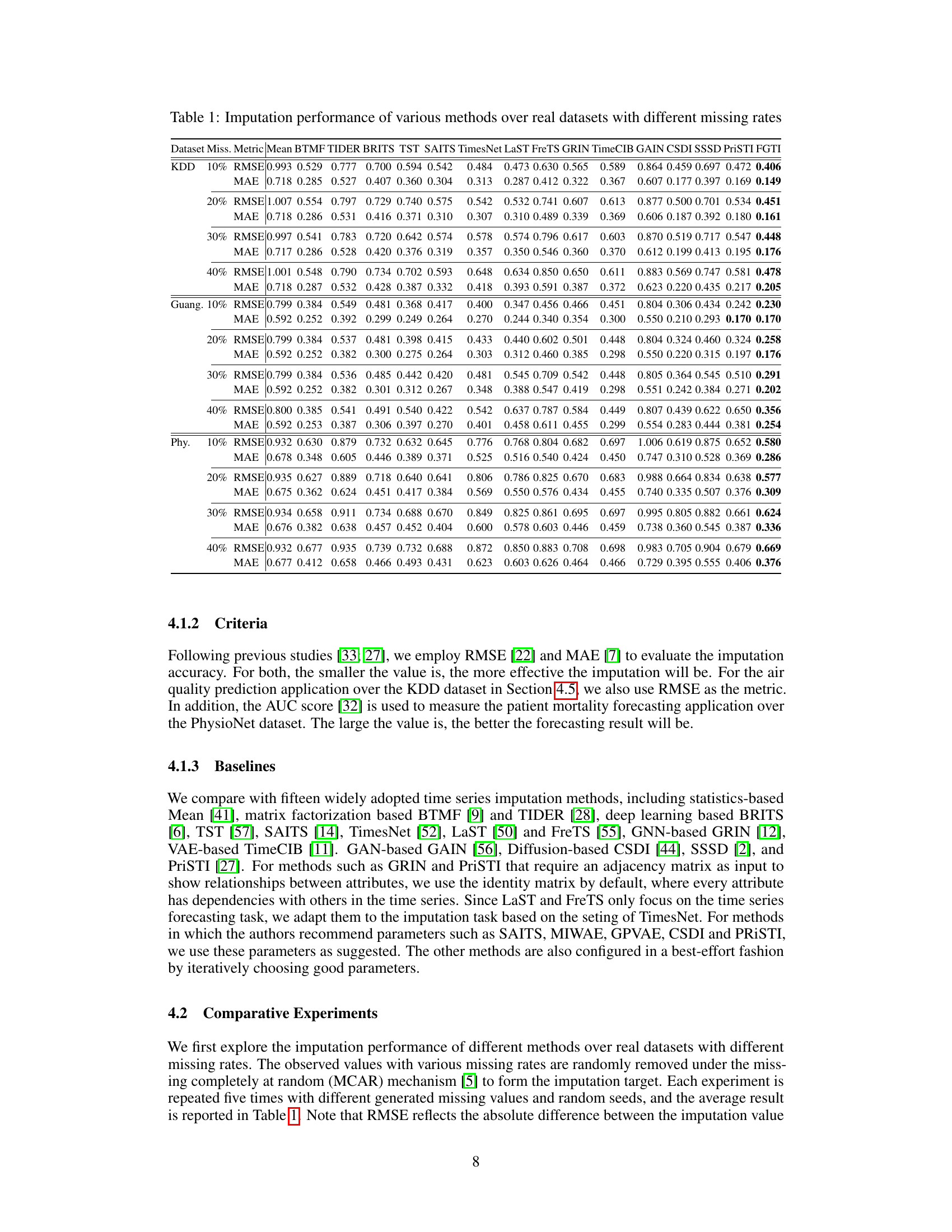
🔼 This table presents the results of a comparative study evaluating the performance of various time series imputation methods on three real-world datasets with varying missing data rates. The methods are compared using two metrics: RMSE (Root Mean Squared Error) and MAE (Mean Absolute Error). Lower values indicate better imputation accuracy. The table allows for a comparison of different imputation techniques under different data conditions and missing rates, highlighting their strengths and weaknesses.
read the caption
Table 1: Imputation performance of various methods over real datasets with different missing rates
In-depth insights#
Freq-aware Imputation#
Frequency-aware imputation methods represent a significant advancement in handling missing data within time series. Traditional methods often struggle with the complexities of multivariate time series, particularly concerning the accurate imputation of residual components. Frequency-aware approaches address this by incorporating frequency-domain information, leveraging the unique spectral characteristics of the data. This allows for a more nuanced understanding of the underlying patterns and improved reconstruction of missing values. By decomposing time series into trend, seasonal, and residual components, these methods can selectively focus on the frequency bands most relevant to each component. This targeted approach is particularly effective in handling high-frequency noise or irregular fluctuations often responsible for substantial imputation errors. The use of filters, such as high-frequency and dominant-frequency filters, allows for the selective enhancement or suppression of specific frequency components. These techniques improve accuracy and also make better use of available information. Cross-domain representation learning further enhances performance by seamlessly integrating frequency and time-domain insights, leading to more robust and accurate imputation models. The benefits extend beyond simple data completion, leading to improvements in downstream tasks like forecasting and anomaly detection.
Cross-domain Learning#
Cross-domain learning, in the context of multivariate time series imputation, is a crucial technique for effectively integrating information from different data domains. FGTI leverages this by combining time-domain and frequency-domain representations. This fusion allows the model to capture both temporal dependencies and frequency-related patterns, which are vital for accurate imputation, especially of the residual term. Time-frequency and attribute-frequency representation learning modules facilitate this integration. By cross-referencing features across these domains, the model gains a more comprehensive understanding of the underlying data structure, leading to improved imputation performance in both accuracy and downstream applications. The key advantage lies in mitigating the limitations of deep learning models in handling high-frequency components, often responsible for significant imputation errors. The success of this approach underscores the importance of considering data from multiple perspectives to overcome the challenges of incomplete multivariate time series data.
Diffusion Model Use#
The utilization of diffusion models in this research is a crucial element for achieving high-quality imputation of multivariate time series data. The core idea lies in leveraging the inherent ability of diffusion models to effectively capture the complex, high-dimensional probability distributions underlying the data. By carefully designing the model architecture and incorporating frequency-domain information, the authors enhance the diffusion model’s capacity to accurately handle noise, missing data, and intricate temporal dependencies. The frequency-aware generative model (FGTI) effectively uses high-frequency and dominant-frequency filters to capture relevant information across different frequency spectrums. This results in a more nuanced and accurate imputation of the residual, trend, and seasonal components. The cross-domain representation learning module, incorporating time and frequency information, further boosts model performance. This approach demonstrates the potential of diffusion models to address the challenges presented by missing data in multivariate time series, surpassing traditional methods in both imputation accuracy and downstream applications.
Ablation Study Done#
An ablation study systematically removes components of a model to assess their individual contributions. In the context of a time series imputation model, this might involve removing specific modules like the high-frequency filter, dominant-frequency filter, or cross-domain representation learning components. By comparing the model’s performance with and without these features, researchers can quantify the impact of each component on overall accuracy. A well-designed ablation study should reveal which aspects are crucial for achieving strong results and highlight potential areas for future improvements or alternative designs. The results could show, for instance, that the high-frequency filter is particularly important for imputing residual terms, while the dominant-frequency filter is more relevant for trend and seasonal components. This detailed analysis allows for a nuanced understanding of the model’s inner workings and provides valuable insights into its strengths and limitations. Moreover, it helps establish the relative importance of each component, possibly suggesting strategies for resource optimization or future research directions.
Real-world Datasets#
The utilization of real-world datasets is crucial for evaluating the effectiveness and generalizability of time series imputation models. These datasets, unlike synthetically generated ones, contain inherent complexities such as noise, missing data patterns, and diverse data distributions that reflect real-world scenarios. Real-world datasets enable a more robust assessment of model performance, moving beyond idealized simulations and providing insights into how algorithms handle the challenges of less-than-perfect data. The selection of datasets should be carefully considered, ensuring they represent the target application and include sufficient diversity in terms of data characteristics and missing data mechanisms. Analyzing model performance across multiple real-world datasets is key to establishing confidence in the models’ ability to generalize across various contexts. The results obtained from real-world data evaluation provide valuable insights into the practical applicability and limitations of the proposed models. A thorough description of the datasets, including data characteristics, data acquisition methods, and missing data mechanisms, is important for reproducibility and allows other researchers to evaluate the findings in the context of their own applications. Furthermore, comparisons with existing methods on the same real-world datasets allows a fair and comprehensive performance evaluation. By carefully choosing and analyzing the results on real-world datasets, researchers can enhance the credibility and impact of their time series imputation models.
More visual insights#
More on figures
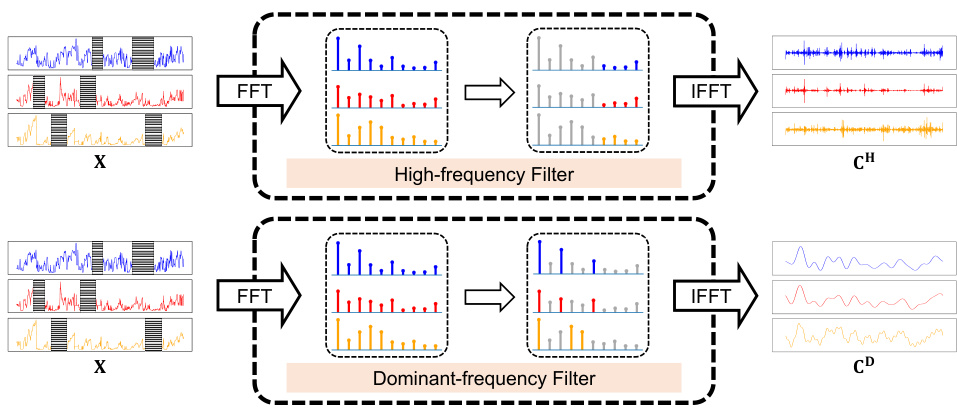
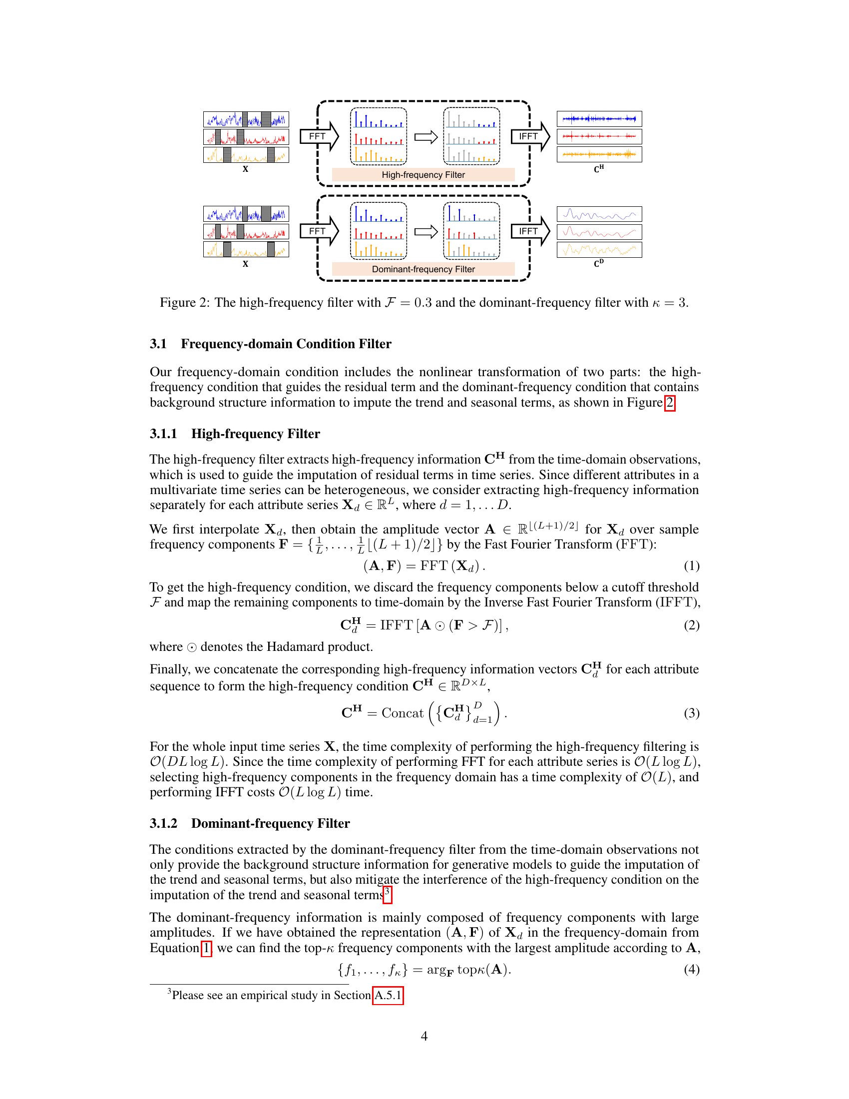
🔼 This figure illustrates the process of extracting frequency-domain information from a time series using two types of filters: high-frequency filter and dominant-frequency filter. The top half shows the steps involved in the high-frequency filtering process, which includes performing a Fast Fourier Transform (FFT) on the input time series, selecting high-frequency components above a threshold (F = 0.3 in this example), and performing an Inverse Fast Fourier Transform (IFFT) to map these components back to the time domain, resulting in the high-frequency condition CH. The bottom half shows a similar process for the dominant-frequency filtering, which identifies the top κ (κ = 3 in this example) frequency components with the largest amplitudes, maps them to the time domain using IFFT, producing the dominant-frequency condition CD. The visual representation uses color-coded bars to represent frequency components and waveforms to represent time series data, illustrating how the filters select and transform the data.
read the caption
Figure 2: The high-frequency filter with F = 0.3 and the dominant-frequency filter with κ = 3.

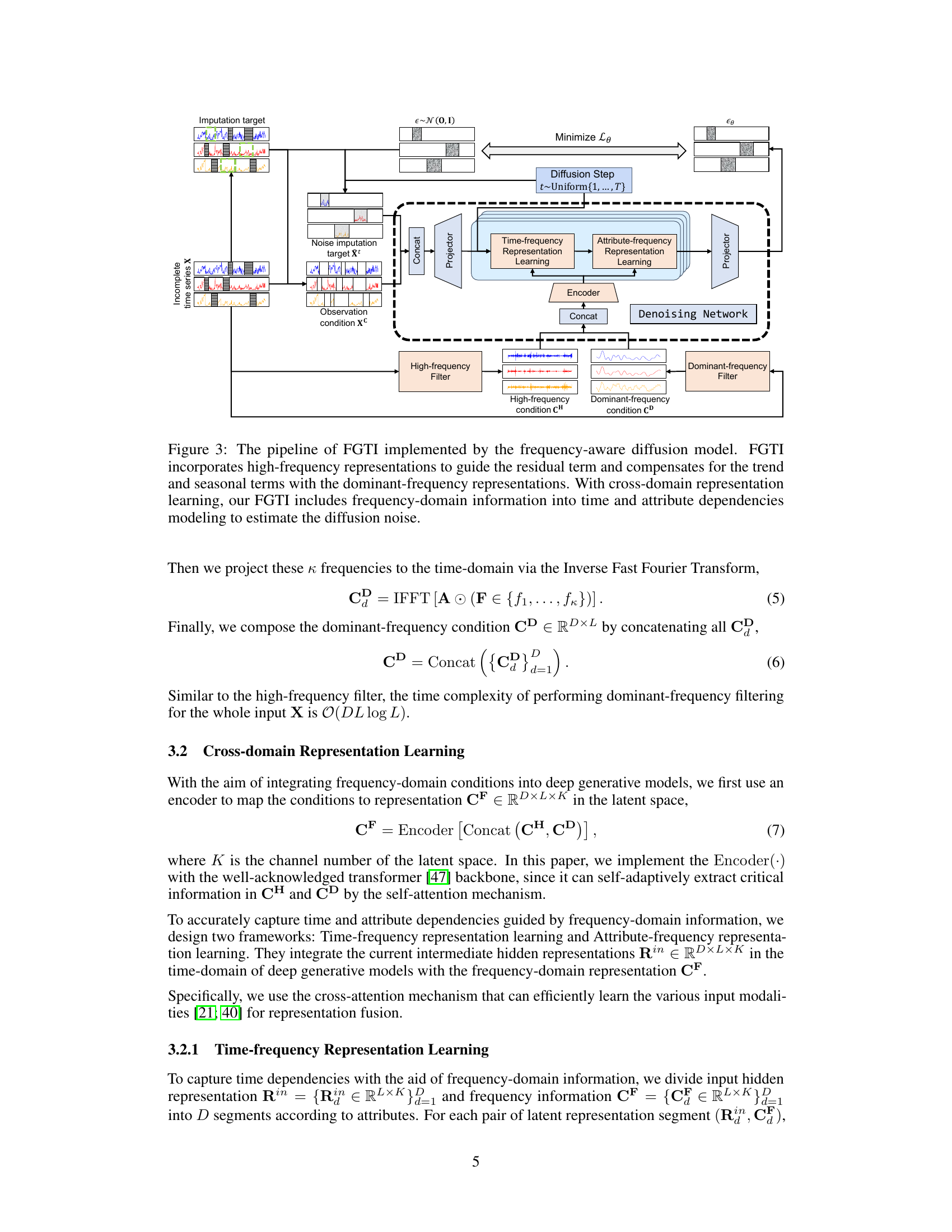
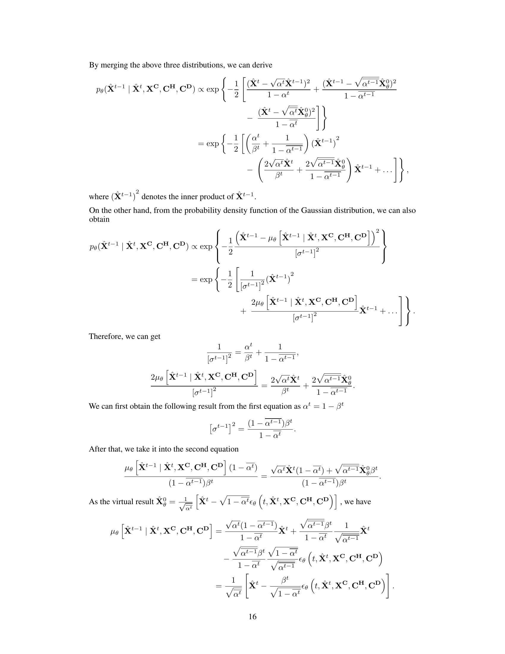
🔼 This figure illustrates the architecture of the Frequency-aware Generative Model for Multivariate Time Series Imputation (FGTI) using a diffusion model. The FGTI model takes incomplete multivariate time series data as input and aims to impute the missing values. It leverages both time-domain and frequency-domain information for improved imputation accuracy. The process starts with a high-frequency filter extracting high-frequency components crucial for residual term imputation and a dominant-frequency filter extracting dominant frequencies for trend and seasonal components. A cross-domain representation learning module combines both frequency-domain features with deep time-domain representations using an encoder and two cross-attention mechanisms (Time-frequency and Attribute-frequency representation learning). Finally, a denoising network utilizes this combined information to generate imputed values, minimizing the diffusion noise.
read the caption
Figure 3: The pipeline of FGTI implemented by the frequency-aware diffusion model. FGTI incorporates high-frequency representations to guide the residual term and compensates for the trend and seasonal terms with the dominant-frequency representations. With cross-domain representation learning, our FGTI includes frequency-domain information into time and attribute dependencies modeling to estimate the diffusion noise.

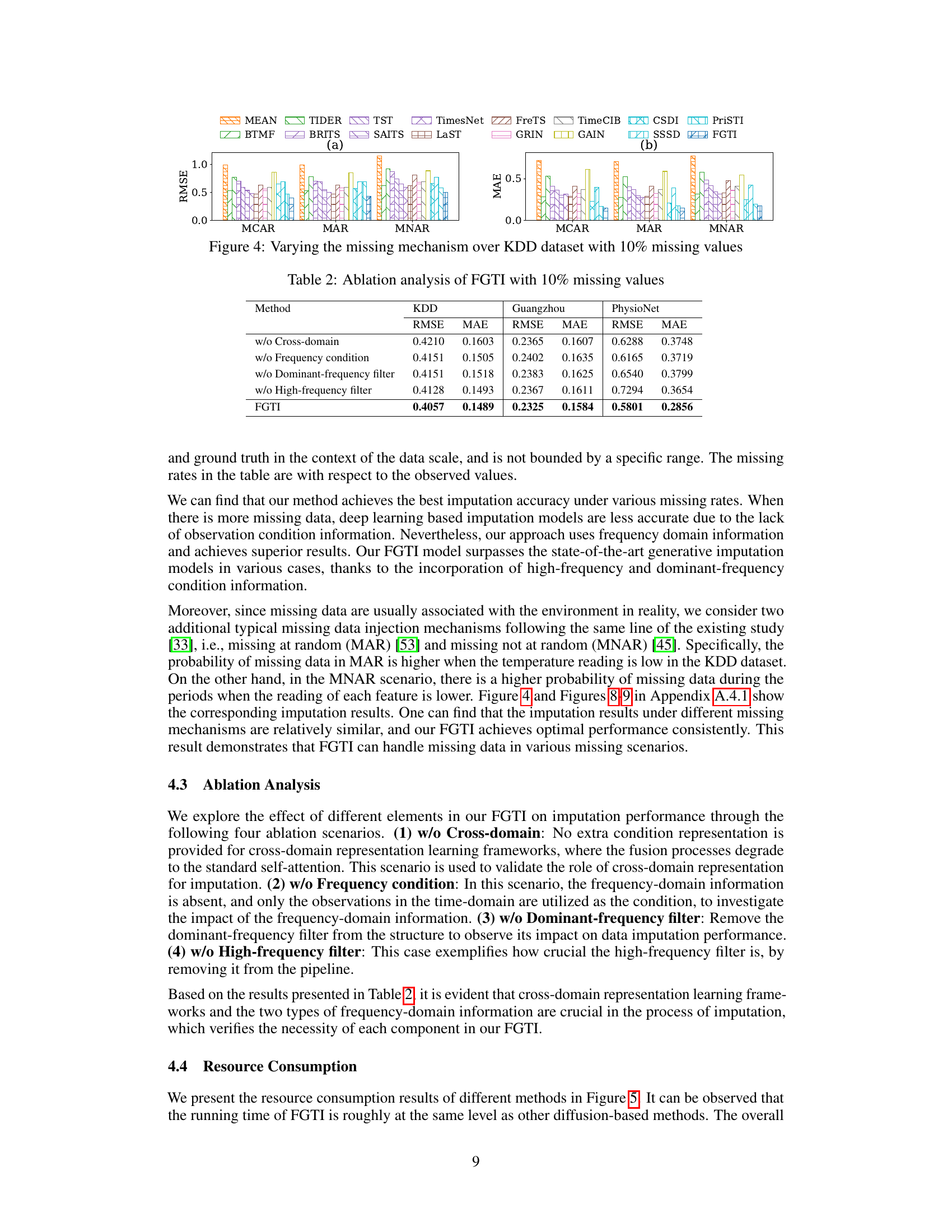
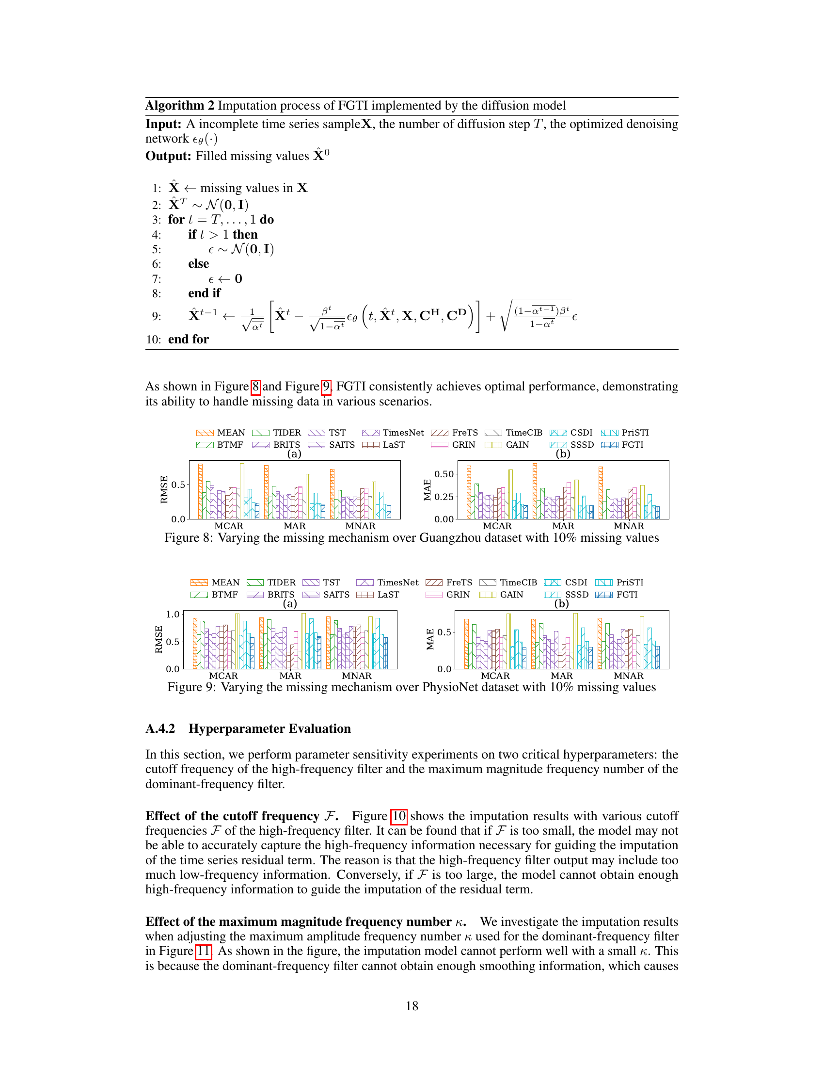
🔼 The figure shows the performance of various imputation methods under different missing mechanisms (MCAR, MAR, MNAR) on the KDD dataset with 10% missing values. The results are presented as RMSE and MAE. It visually demonstrates the robustness of FGTI across various missing data scenarios.
read the caption
Figure 4: Varying the missing mechanism over KDD dataset with 10% missing values
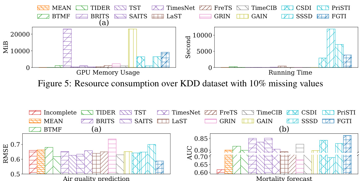
🔼 This figure shows the GPU memory usage and running time of various imputation methods on the KDD dataset with 10% missing values. FGTI’s resource consumption is comparable to other diffusion-based methods, demonstrating reasonable efficiency despite its superior accuracy.
read the caption
Figure 5: Resource consumption over KDD dataset with 10% missing values
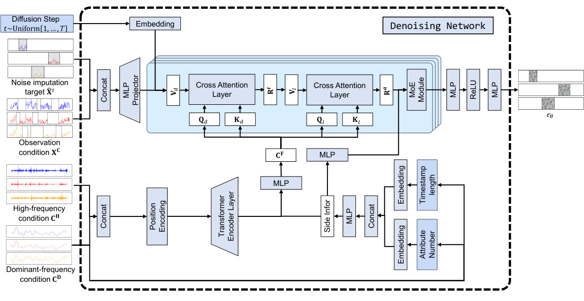
🔼 This figure illustrates the architecture of the Frequency-aware Generative Models for Multivariate Time Series Imputation (FGTI) method. It shows how the model uses both time-domain and frequency-domain information (high-frequency and dominant-frequency components) to guide the imputation process within a diffusion model framework. The high-frequency information focuses on improving the residual imputation, while the dominant-frequency information helps impute trend and seasonal components. Cross-domain representation learning modules combine these insights to estimate the diffusion noise accurately.
read the caption
Figure 3: The pipeline of FGTI implemented by the frequency-aware diffusion model. FGTI incorporates high-frequency representations to guide the residual term and compensates for the trend and seasonal terms with the dominant-frequency representations. With cross-domain representation learning, our FGTI includes frequency-domain information into time and attribute dependencies modeling to estimate the diffusion noise.
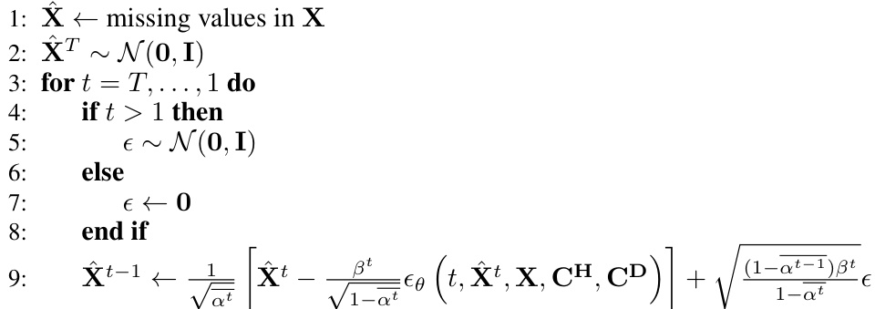
🔼 This figure shows the architecture of the Frequency-aware Generative Models for Multivariate Time Series Imputation (FGTI) model. FGTI uses a diffusion model framework and incorporates frequency-domain information (high-frequency and dominant-frequency components) to improve imputation accuracy, particularly for the residual term. The model leverages cross-domain representation learning to fuse time-domain and frequency-domain information for enhanced performance.
read the caption
Figure 3: The pipeline of FGTI implemented by the frequency-aware diffusion model. FGTI incorporates high-frequency representations to guide the residual term and compensates for the trend and seasonal terms with the dominant-frequency representations. With cross-domain representation learning, our FGTI includes frequency-domain information into time and attribute dependencies modeling to estimate the diffusion noise.

🔼 The figure shows a bar chart comparing the imputation accuracy of three different components of multivariate time series data (trend, seasonal, and residual) using various imputation methods. The results reveal that the residual term has the highest imputation error among the three components, indicating that improving the imputation accuracy of the residual term is crucial for enhancing the overall imputation performance.
read the caption
Figure 1: Improving the imputation accuracy of the residual term is the key to boosting the imputation performance of the model.

🔼 This figure displays the impact of varying the cutoff frequency (F) of the high-frequency filter on imputation accuracy, measured by RMSE and MAE. The results are shown for three datasets (KDD, Guangzhou, and PhysioNet). It demonstrates the importance of selecting an appropriate cutoff frequency, as both too low and too high values negatively affect performance. A mid-range value for F seems to produce optimal results.
read the caption
Figure 10: Varying the cutoff frequency F of the high-frequency filter with 10% missing values

🔼 This figure shows the impact of the hyperparameter κ (maximum magnitude frequency number) in the dominant-frequency filter on the imputation performance. The x-axis represents different values of κ, and the y-axis shows the RMSE and MAE values for three different datasets (KDD, Guangzhou, and PhysioNet). The results show an optimal range for κ. Values that are too low might prevent accurate capture of dominant frequency components while values that are too high might introduce high-frequency information interfering with imputation of trend and seasonal components.
read the caption
Figure 11: Varying the number of maximum magnitude frequency of the dominant-frequency filter with 10% missing values

🔼 This figure shows a bar chart comparing the imputation accuracy of three components (trend, seasonal, and residual) of a time series using different imputation methods. The key finding is that the residual term has significantly higher imputation error compared to the trend and seasonal components. This highlights the importance of accurately imputing the residual term for achieving better overall imputation performance.
read the caption
Figure 1: Improving the imputation accuracy of the residual term is the key to boosting the imputation performance of the model.
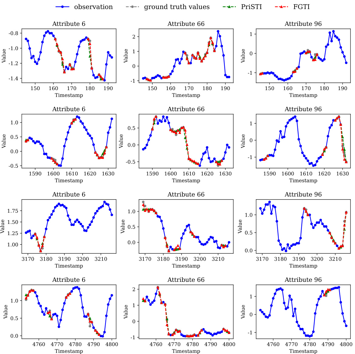
🔼 This figure shows a bar chart comparing the imputation accuracy of three different components of time series data (trend, seasonal, and residual) using various imputation methods on the KDD dataset. The results reveal that the residual term has significantly higher imputation error compared to the trend and seasonal terms, highlighting the importance of accurately imputing the residual term for overall improved imputation performance. The figure also shows line plots illustrating examples of the three time series components (trend, seasonal, and residual) and how well FGTI performs compared to PriSTI in estimating them.
read the caption
Figure 1: Improving the imputation accuracy of the residual term is the key to boosting the imputation performance of the model.
More on tables

🔼 This table presents the ablation study results for the Frequency-aware Generative Models for Multivariate Time Series Imputation (FGTI) model. The study evaluates the impact of removing different components of the FGTI model on the imputation performance using RMSE and MAE metrics across three datasets (KDD, Guangzhou, and PhysioNet). By systematically removing components such as cross-domain learning, frequency condition, dominant-frequency filter, and high-frequency filter, the table reveals the relative contribution of each component to the overall accuracy of the model.
read the caption
Table 2: Ablation analysis of FGTI with 10% missing values
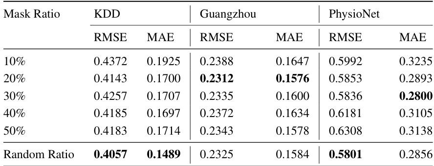
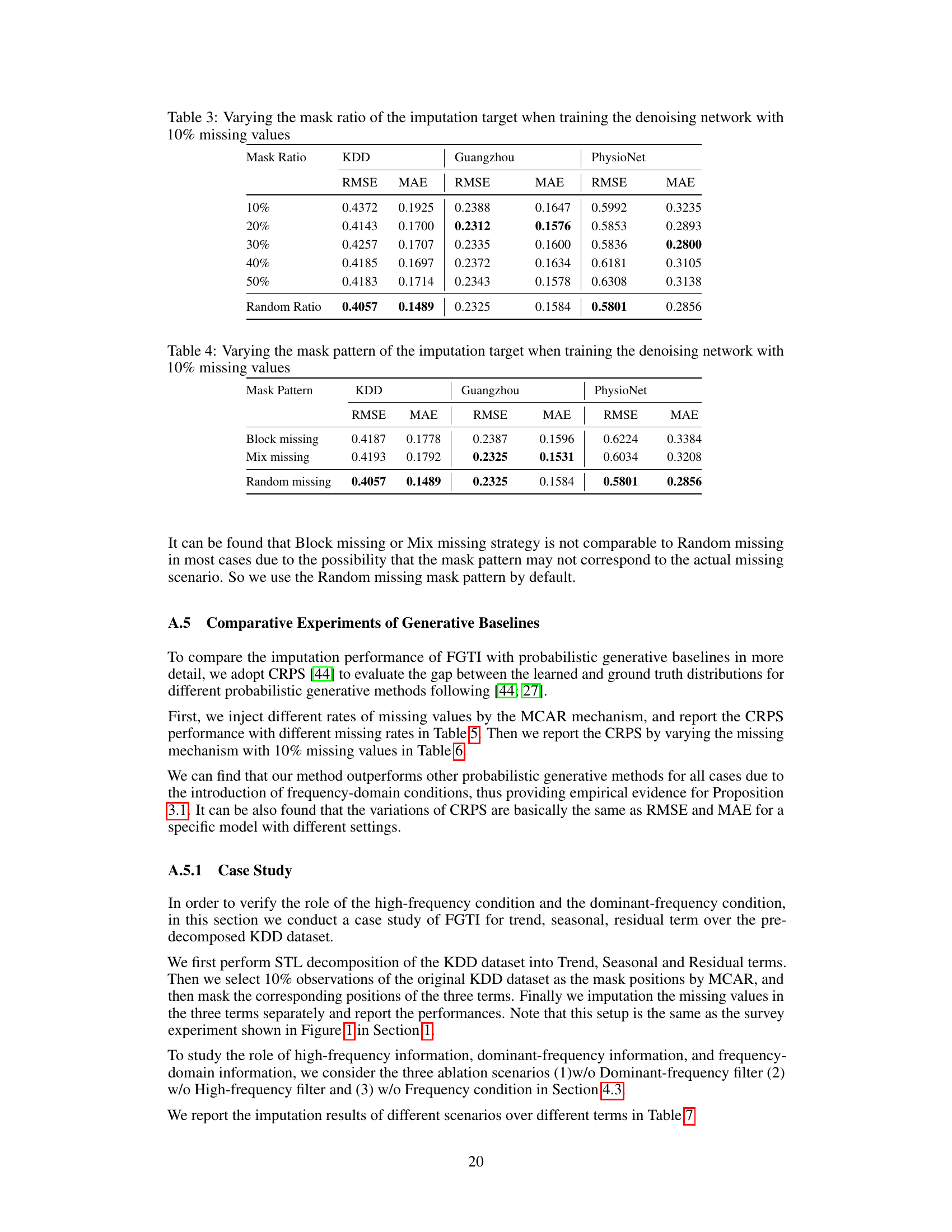
🔼 This table presents the imputation performance (RMSE and MAE) of the FGTI model on three datasets (KDD, Guangzhou, and PhysioNet) with varying mask ratios (10%, 20%, 30%, 40%, 50%, and random ratio) during the training of the denoising network. The mask ratio represents the percentage of observed values used as the imputation target. A random ratio means a different ratio is used at each training step, instead of a fixed masking ratio. The table shows how the imputation accuracy changes with different mask ratios for each dataset.
read the caption
Table 3: Varying the mask ratio of the imputation target when training the denoising network with 10% missing values

🔼 This table presents the imputation performance (RMSE and MAE) of the FGTI model trained with different mask patterns (block missing, mix missing, random missing) on three datasets (KDD, Guangzhou, PhysioNet). The goal is to evaluate the impact of the mask pattern on the model’s ability to impute missing values when 10% of the data is missing.
read the caption
Table 4: Varying the mask pattern of the imputation target when training the denoising network with 10% missing values

🔼 This table presents the results of several imputation methods on three real-world datasets with varying missing data rates (10%, 20%, 30%, and 40%). The methods are compared using RMSE and MAE metrics to assess imputation accuracy. The datasets used are KDD, Guangzhou, and PhysioNet, each representing a different type of multivariate time series data. The table allows for a comparison of the effectiveness of different approaches in handling missing data across different datasets and missing rates.
read the caption
Table 1: Imputation performance of various methods over real datasets with different missing rates

🔼 This table presents the Continuous Ranked Probability Score (CRPS) for various probabilistic generative models under different missing data mechanisms (MCAR, MAR, MNAR). The CRPS evaluates the discrepancy between predicted and actual probability distributions. Lower CRPS values indicate better performance.
read the caption
Table 6: CRPS of various probabilistic generative methods with different missing mechanisms

🔼 This table presents the imputation results (RMSE and MAE) for the trend, seasonal, and residual components of the KDD dataset when 10% of the data is missing. It compares the performance of the FGTI model against three ablation studies: removing the frequency condition, removing the dominant-frequency filter, and removing the high-frequency filter. The results show the impact of each component (high-frequency, dominant-frequency, and frequency condition) on the accuracy of imputing each of the three time series components.
read the caption
Table 7: Imputation results for the trend, seasonal and residual terms of KDD dataset with 10% missing values
Full paper#
