Improving Adaptivity via Over-Parameterization in Sequence Models

↗ arXiv ↗ Hugging Face ↗ Chat

TL;DR

#

Key Takeaways

#

Why does it matter?

#

This paper is crucial because it challenges the conventional understanding of neural network training by demonstrating that over-parameterization, a common practice, can significantly improve adaptability and generalization. It provides a novel perspective on over-parameterization’s benefits, which is relevant to the current focus on understanding the efficiency and generalization capabilities of neural networks. The research opens new avenues for investigating the dynamic interplay between network architecture, initialization, and optimization processes, which is essential for developing more efficient and adaptive AI models.

Visual Insights

#

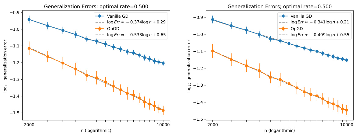
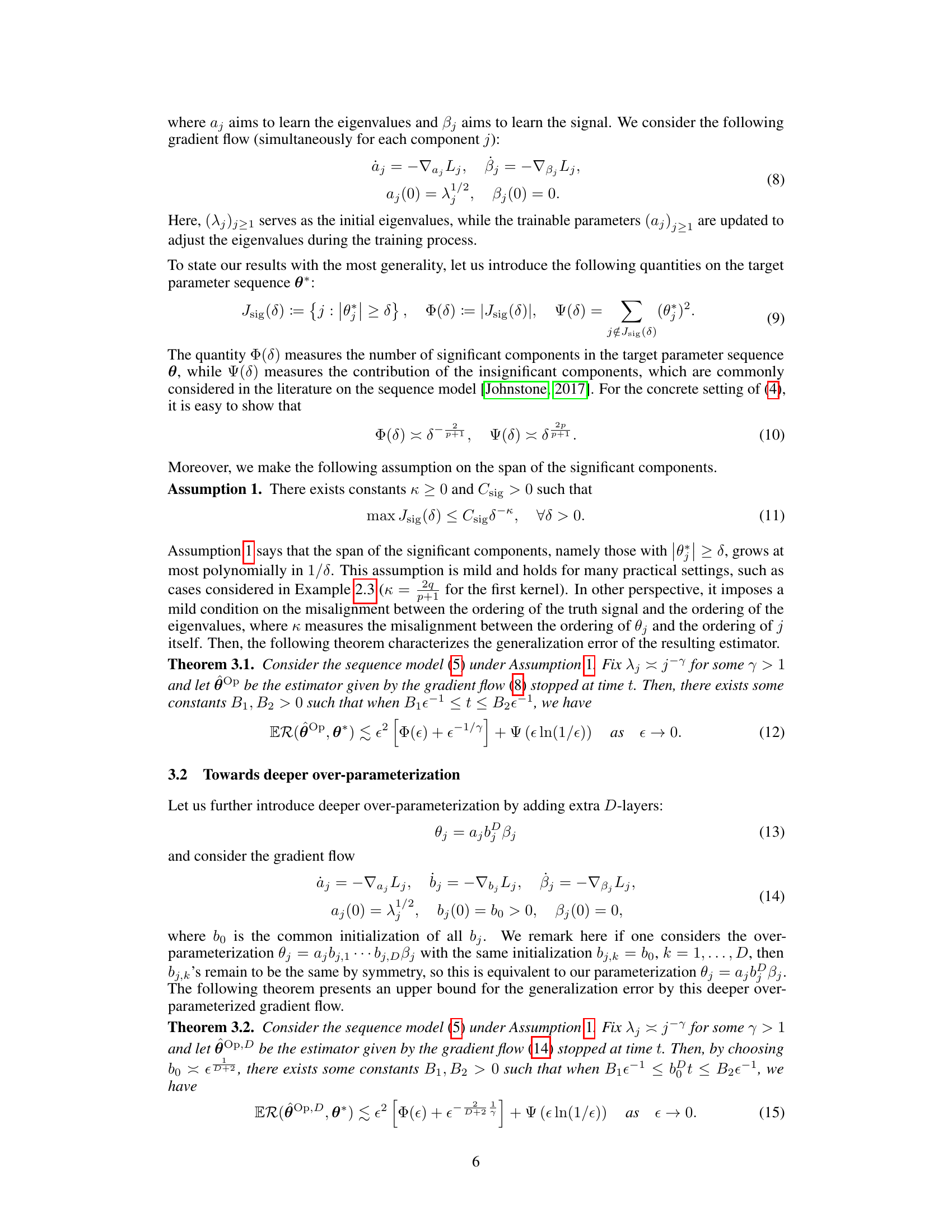
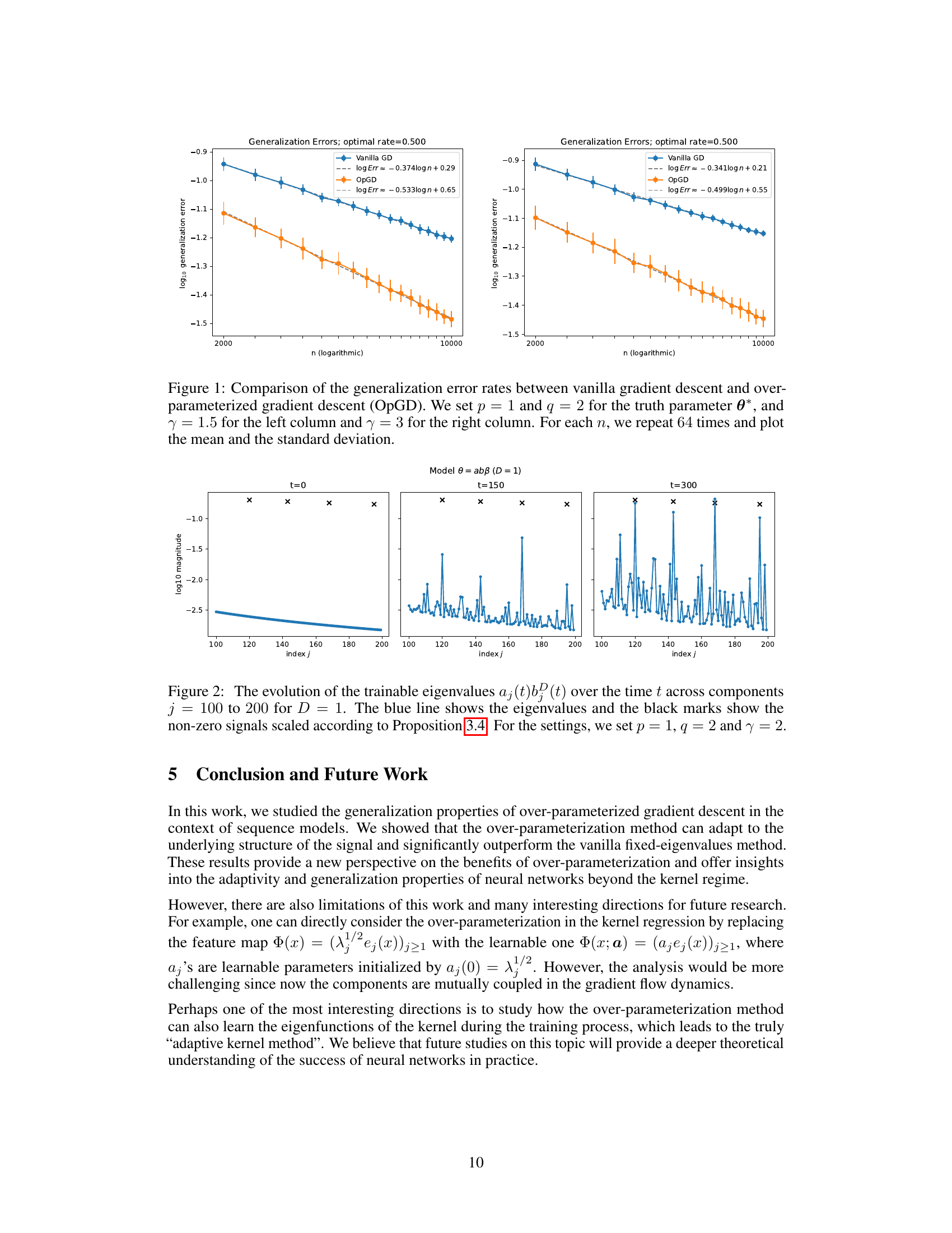
🔼 This figure compares the generalization error rates of vanilla gradient descent and over-parameterized gradient descent (OpGD) for different sample sizes (n). Two different eigenvalue decay rates (γ = 1.5 and γ = 3) are considered. The results demonstrate that OpGD achieves a better generalization performance compared to the vanilla gradient descent method, especially when the misalignment between the eigenvalues and the true signal is more severe (larger q). The error bars represent the standard deviation across multiple runs.

read the caption

Figure 1: Comparison of the generalization error rates between vanilla gradient descent and over-parameterized gradient descent (OpGD). We set p = 1 and q = 2 for the truth parameter θ*, and γ = 1.5 for the left column and γ = 3 for the right column. For each n, we repeat 64 times and plot the mean and the standard deviation.

🔼 This table presents the convergence rates of the over-parameterized gradient descent method for different settings of parameters p, q, and γ. The convergence rate, estimated via logarithmic least-squares fitting, shows the relationship between the generalization error and the sample size (n). The ideal convergence rate (r*) is also provided for comparison. Each rate is an average of 256 repetitions.

read the caption

Table 1: Convergence rates of the over-parameterized gradient descent (8) under different settings of the truth parameter p, q and the eigenvalue decay rate γ, where r* is the ideal convergence rate. The convergence rate is estimated by the logarithmic least-squares fitting of the generalization error with n ranging from 2000, 2200,..., 4000, where the generalization error is the mean of 256 repetitions.

In-depth insights

#

Over-parameterization

#

The concept of over-parameterization, explored in the context of sequence models, reveals a surprising capacity for improved model adaptability and generalization. Contrary to traditional kernel regression methods, which rely on fixed kernels, over-parameterization introduces a dynamic adjustment of eigenvalues during training. This dynamic adaptation allows the model to effectively learn the underlying structure of the signal, leading to superior performance compared to methods with fixed eigenvalues. The research highlights that deeper over-parameterization can further enhance generalization capabilities, offering a novel perspective on the potential of neural networks beyond the limitations of the kernel regime. Early stopping plays a critical role in the success of this method, mitigating overfitting and ensuring optimal convergence rates. The findings challenge traditional assumptions and present a valuable new theoretical framework for understanding the effectiveness of neural network training.

Sequence Model

#

The heading ‘Sequence Model’ suggests a focus on applying the research to sequential data. This is a significant choice, as sequence models capture temporal dependencies, which are crucial in many real-world applications such as natural language processing, time series analysis, and speech recognition. The paper likely uses a sequence model framework to illustrate the advantages of over-parameterization for improving adaptivity and generalization. The choice of a sequence model offers a simplified yet powerful setting to explore this; it allows the researchers to focus on the core concepts of eigenvalue adjustment and gradient descent without the complexities of other non-parametric approaches. The theoretical analysis within the ‘Sequence Model’ section likely examines how the over-parameterized gradient flow affects the learning dynamics and generalization capabilities when dealing with temporal information. Furthermore, the results within this section would support claims about the efficacy of the over-parameterization approach itself.

Eigenvalue Adaptivity

#

The concept of “Eigenvalue Adaptivity” in the context of the research paper centers on the dynamic adjustment of eigenvalues during the model training process. Instead of relying on a fixed kernel with predetermined eigenvalues, the proposed method introduces over-parameterization to enable the model to learn and adapt the eigenvalues. This approach addresses the limitations of traditional kernel regression methods, which can suffer from misalignment between the kernel’s eigenvalues and the true underlying signal structure. By learning the eigenvalues, the model can better align itself with the signal, leading to improved generalization and prediction accuracy. The theoretical analysis highlights the benefits of this adaptive eigenvalue adjustment, particularly in situations with severe misalignment or low-dimensional structure within the data. The effectiveness of this approach is further enhanced by using deeper over-parameterization, which increases the model’s capacity to learn complex relationships and mitigate overfitting. This concept demonstrates how the ability to adapt eigenvalues during learning is crucial for overcoming the limitations of fixed-kernel methods and opens up opportunities for creating more adaptable and generalizable models.

Generalization Bounds

#

Generalization bounds in machine learning aim to quantify the difference between a model’s performance on training data and its performance on unseen data. Tight generalization bounds are crucial for understanding model robustness and preventing overfitting. They provide theoretical guarantees on how well a learned model will generalize to new, previously unseen examples. The derivation of such bounds often involves intricate statistical analysis, leveraging concepts like Rademacher complexity, VC dimension, or covering numbers to characterize the model’s capacity and the complexity of the hypothesis space. Factors like model complexity, data size, and the noise level significantly influence generalization bounds. A model’s capacity affects its ability to fit the training data (and potentially overfit), while data size determines the amount of information available to constrain the model’s learning. Noise, on the other hand, introduces uncertainty that limits how well the model can generalize. The practical utility of generalization bounds is often debated, as they can sometimes be loose and fail to provide practically relevant insights. Nevertheless, the pursuit of tighter bounds and more effective methods for analyzing model generalization remains a central theme in machine learning research, informing the design of models and algorithms that are both efficient and accurate.

Future Directions

#

The research paper’s “Future Directions” section could explore several promising avenues. Extending the over-parameterization approach beyond sequence models to general kernel regression is crucial. This would involve dynamically learning both eigenvalues and eigenfunctions, creating a truly adaptive kernel. Investigating the interplay between over-parameterization, depth, and the generalization performance of neural networks beyond the infinite-width regime is another important direction. This might involve analyzing how over-parameterization affects the dynamic evolution of kernels during training. Theoretically analyzing the adaptive choice of stopping time in over-parameterized gradient descent is also important, potentially leading to universally optimal stopping rules. Finally, empirical validation on a wider range of datasets and network architectures, including those with complex data dependencies, would be necessary to demonstrate the practical significance of over-parameterization.

More visual insights

#

More on figures

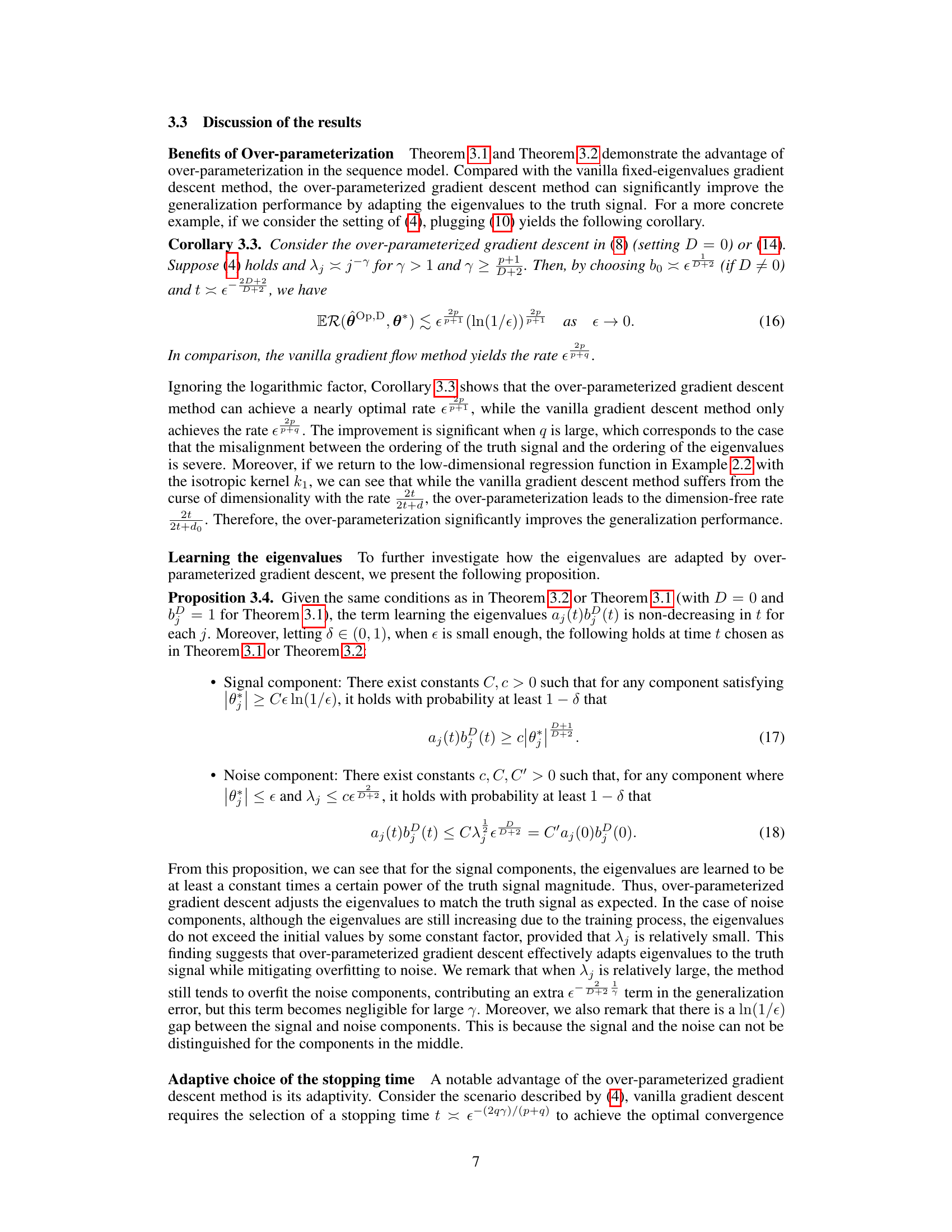
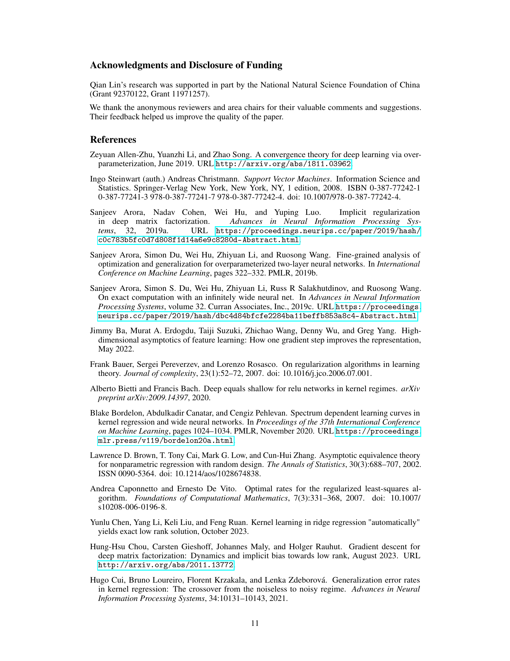
🔼 This figure shows the generalization error for three different over-parameterized models (D=0, 1, and 3) across various training times (t). It also illustrates how the trainable eigenvalues (aj(t)b(t)) evolve over time for a subset of components (j=100 to 200). The plot highlights the adaptive nature of the eigenvalues, showing how they adjust to both signal and noise components according to the theoretical proposition 3.4. The settings used for this experiment are p=1, q=2, and γ=2.

read the caption

Figure 4: The generalization error as well as the evolution of the eigenvalue terms a_j(t)b(t) over the time t. The first row shows the generalization error of three parameterizations D = 0,1,3 with respect to the training time t. The rest of the rows show the evolution of the eigenvalue terms a_j(t)b(t) over the time t. For presentation, we select the index j = 100 to 200. The blue line shows the eigenvalue terms and the black marks show the non-zero signals scaled according to Proposition 3.4. For the settings, we set p = 1, q = 2 and y = 2.

🔼 This figure compares the generalization error rates of vanilla gradient descent and the over-parameterized gradient descent method proposed in the paper. Two different values of γ (1.5 and 3) are used, resulting in four subplots. Each subplot shows the generalization error (log scale) versus the sample size (log scale) for each method. Error bars representing standard deviations are included for 64 repetitions per data point. The results demonstrate that the over-parameterized method consistently achieves a lower generalization error across different γ values.

read the caption

Figure 1: Comparison of the generalization error rates between vanilla gradient descent and over-parameterized gradient descent (OpGD). We set p = 1 and q = 2 for the truth parameter θ*, and γ = 1.5 for the left column and γ = 3 for the right column. For each n, we repeat 64 times and plot the mean and the standard deviation.

🔼 This figure shows the generalization error and eigenvalue evolution for different depths of over-parameterization (D=0, 1, 3). The top row displays the generalization error over time for each depth, while the subsequent rows illustrate the evolution of trainable eigenvalues (aj(t)b(t)D) over time for a subset of components (j=100 to 200). Significant components are highlighted. The results demonstrate how deeper over-parameterization improves generalization and adapts eigenvalues to the signal structure.

read the caption

Figure 4: The generalization error as well as the evolution of the eigenvalue terms a_j(t)b(t)^D over the time t. The first row shows the generalization error of three parameterizations D = 0,1,3 with respect to the training time t. The rest of the rows show the evolution of the eigenvalue terms a_j(t)b(t)^D over the time t. For presentation, we select the index j = 100 to 200. The blue line shows the eigenvalue terms and the black marks show the non-zero signals scaled according to Proposition 3.4. For the settings, we set p = 1, q = 2 and y = 2.

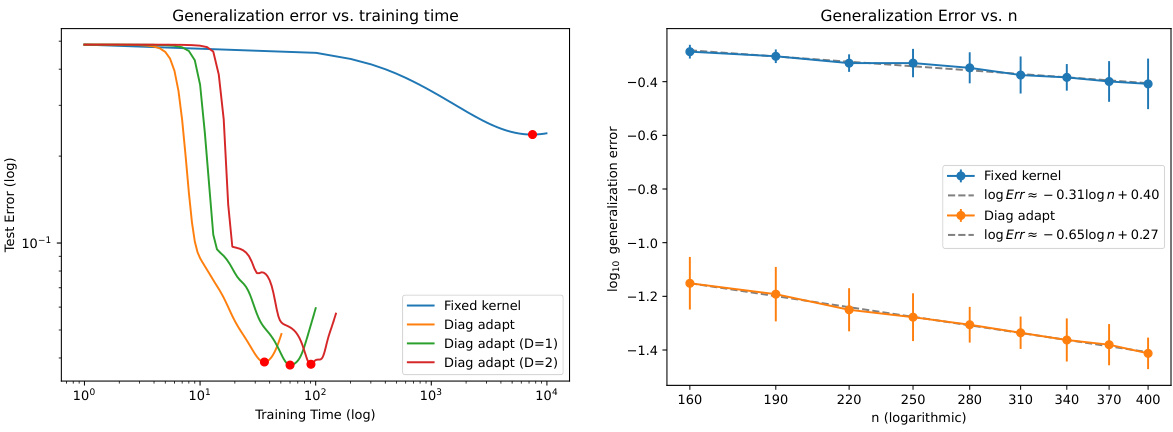
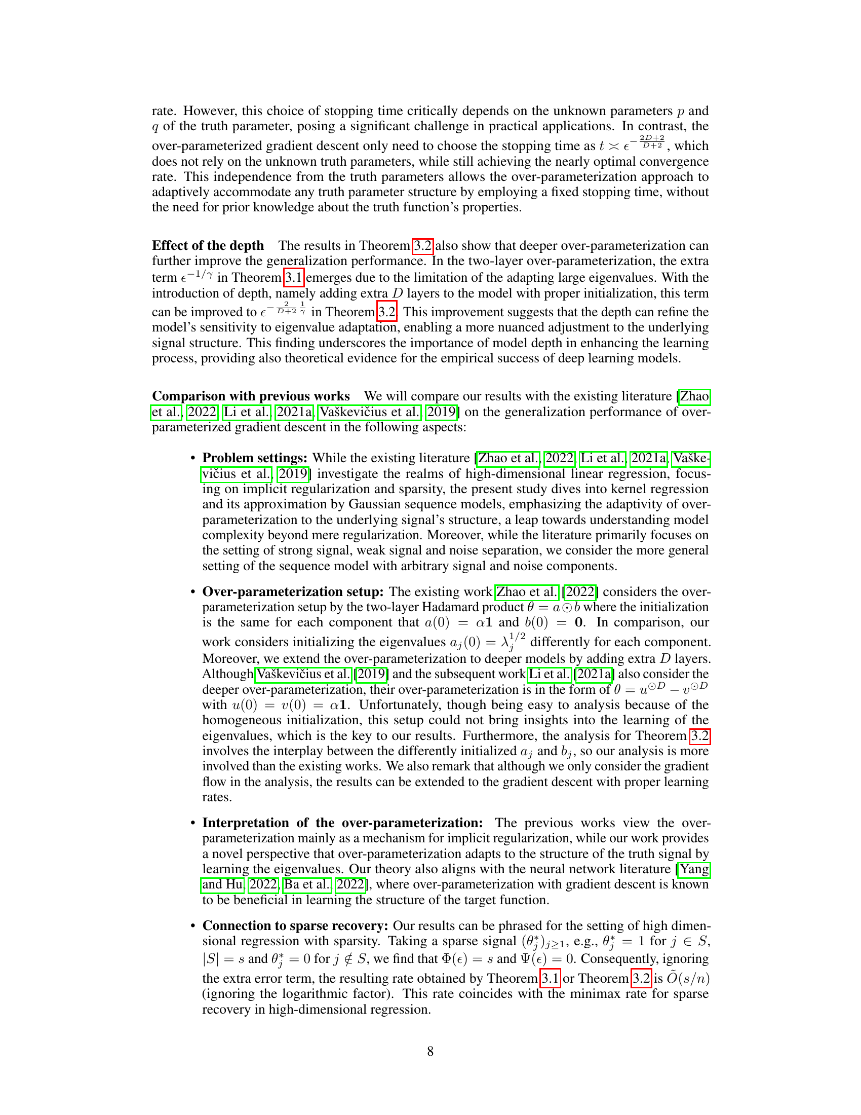
🔼 This figure compares the generalization performance of two methods: the fixed kernel gradient descent and the diagonal adaptive kernel method. The left panel shows the generalization error curves obtained from a single trial of the two methods, illustrating how the diagonal adaptive kernel method achieves a lower generalization error with increased training time. The right panel provides a more comprehensive comparison by plotting the generalization error rate against the sample size (n) for both methods, confirming the superior performance of the diagonal adaptive kernel method in terms of convergence rate.

read the caption

Figure 5: Comparison of the generalization error between the fixed kernel gradient method and the diagonal adaptive kernel method. The left figure shows the generalization error curve of a single trial. The right figure shows the generalization error rates with respect to the sample size n.

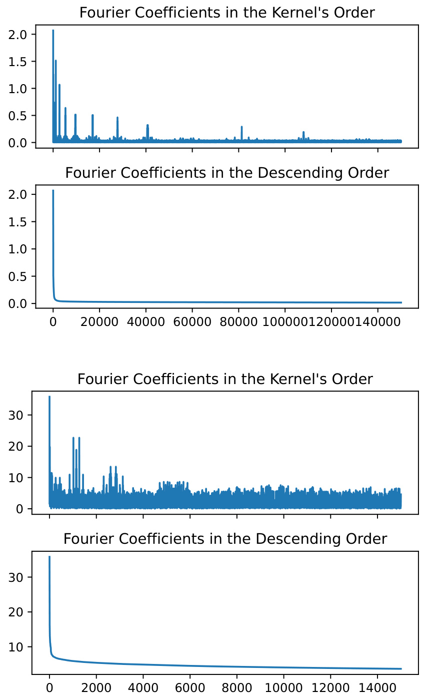
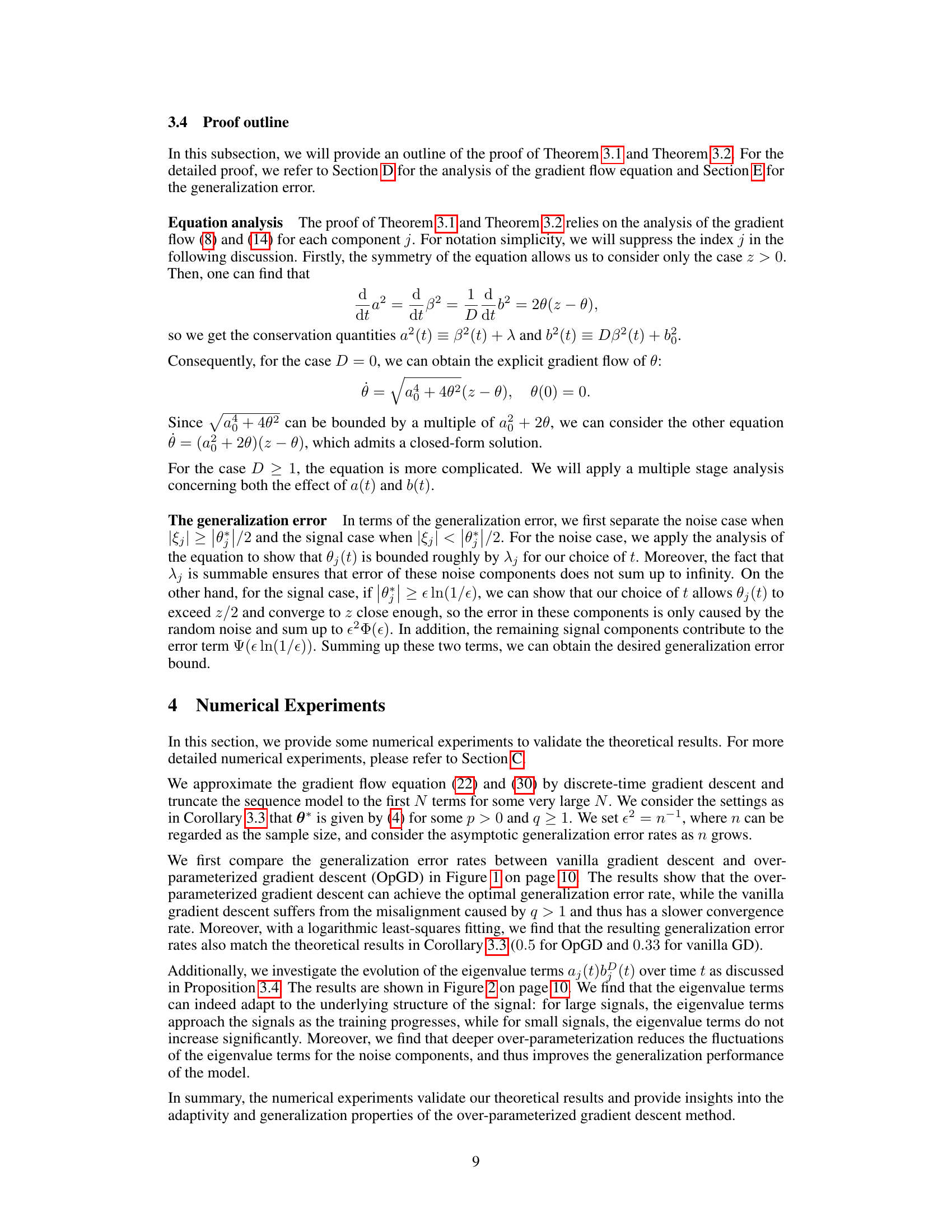
🔼 This figure shows the empirical coefficients of the regression function projected onto the Fourier basis for the 'California Housing' and 'Concrete Compressive Strength' datasets. The top two subfigures correspond to the 'California Housing' dataset, while the bottom two correspond to the 'Concrete Compressive Strength' dataset. In each pair of subfigures, the left one displays the coefficients in the kernel’s order, while the right one shows them sorted in descending order. The plots reveal the distribution of coefficients, highlighting the presence of spikes or large values and a potential mismatch between the kernel eigenvalue order and the order of significance of the coefficients.

read the caption

Figure 6: The empirical coefficients of the regression function over the Fourier basis for the \'California Housing\' dataset (upper) and \'Concrete Compressive Strength\' dataset (lower). Note that we take different numbers of Fourier basis functions for the two datasets for better visualization.

Full paper

#