↗ OpenReview ↗ NeurIPS Homepage ↗ Chat
TL;DR#
Time series forecasting is crucial across numerous domains but existing Transformer-based models suffer from vulnerabilities to high-frequency signals, computational inefficiency, and limitations in full-spectrum utilization. These shortcomings hinder accurate predictions, especially for extensive datasets. The paper addresses these issues by exploring the potential of signal processing techniques in deep time series forecasting.
The proposed FilterNet uses learnable frequency filters to select key temporal patterns. Two types of filters, plain and contextual shaping filters, are introduced. FilterNet effectively surrogates widely adopted linear and attention mappings while achieving robustness against high-frequency noise and utilizing the entire frequency spectrum. Experimental results demonstrate FilterNet’s superior performance in terms of effectiveness and efficiency compared to state-of-the-art methods across eight benchmark datasets.
Key Takeaways#
Why does it matter?#
This paper is important because it introduces a novel approach to time series forecasting that outperforms existing methods. FilterNet leverages frequency filters, a concept borrowed from signal processing, to effectively extract key temporal patterns and handle high-frequency noise. This offers enhanced accuracy and efficiency, opening new avenues for research in deep learning for time series analysis and forecasting.
Visual Insights#

The figure shows the performance comparison of the iTransformer and FilterNet models on a synthetic dataset with low, middle, and high-frequency components. FilterNet significantly outperforms iTransformer, achieving a much lower MSE (Mean Squared Error). This highlights FilterNet’s superior ability to handle multi-frequency signals, which is a key advantage over Transformer-based models that often struggle with high-frequency noise. Appendix C.4 provides additional details regarding experimental setup.
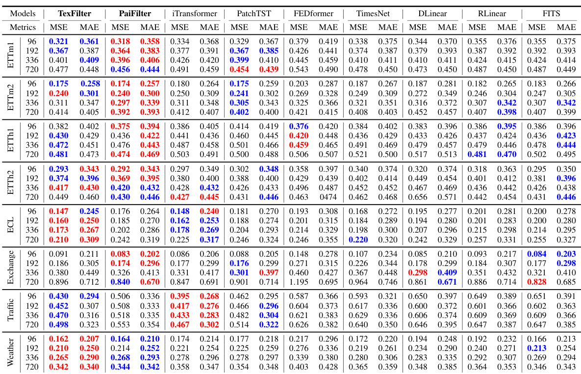
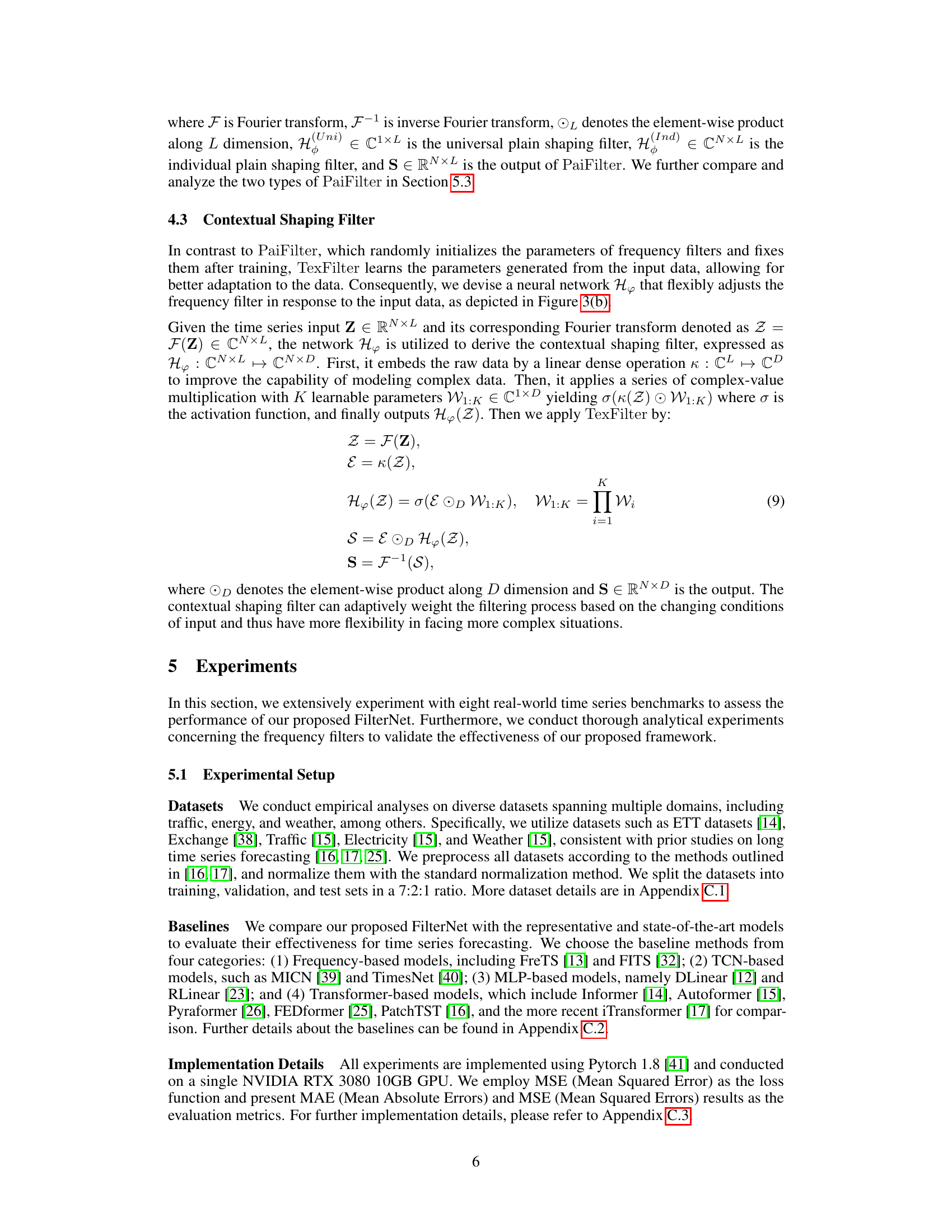
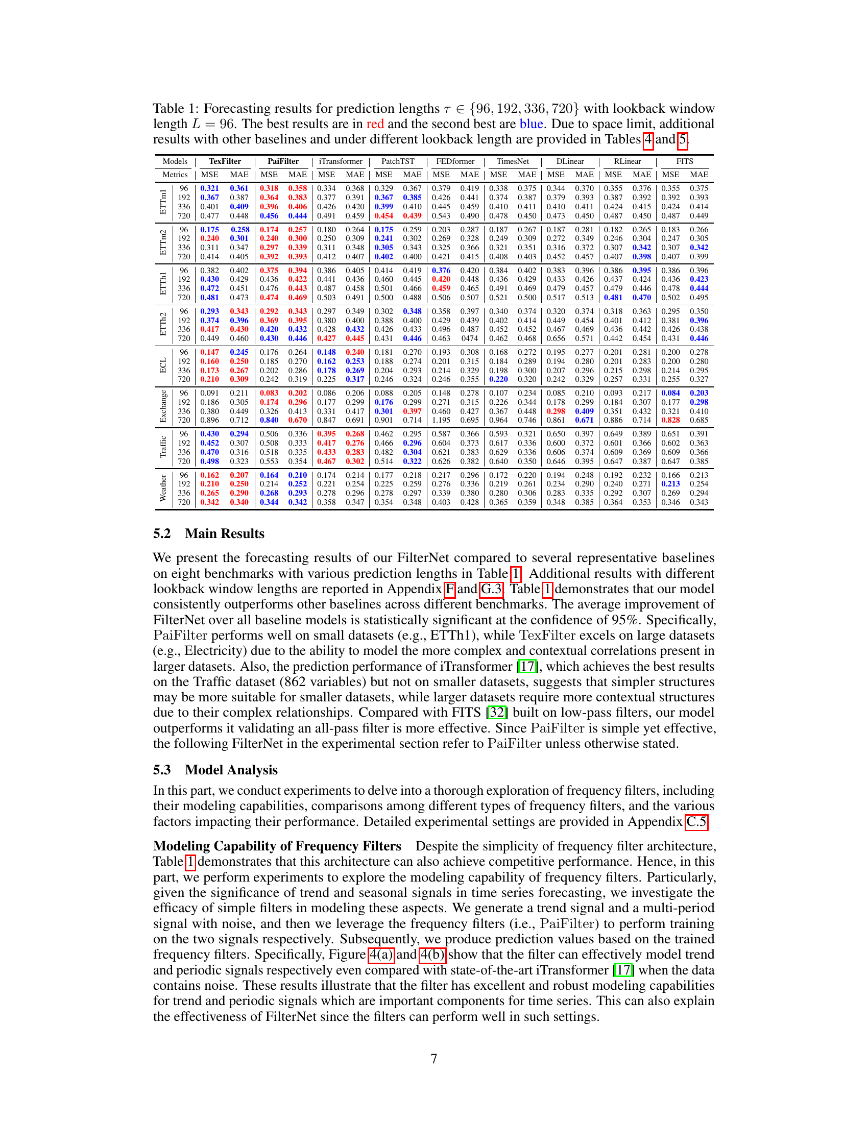
This table presents the forecasting results of the proposed FilterNet model and several other state-of-the-art models on eight benchmark datasets. The results are shown for four different prediction lengths (τ) with a fixed lookback window length (L). The best and second-best results are highlighted in red and blue, respectively. The full results, including those for other baselines and different lookback window lengths, can be found in additional tables within the paper.
In-depth insights#
FilterNet Architecture#
The FilterNet architecture is thoughtfully designed for efficient and effective time series forecasting. It leverages frequency filtering, a signal processing technique, to enhance performance. The core innovation lies in the introduction of learnable frequency filters, specifically the ‘plain shaping filter’ for simpler time series and the ‘contextual shaping filter’ for more complex ones. These filters offer selective attenuation and passing of frequency components which are crucial for accurate predictions. Instance normalization is incorporated to handle the non-stationarity commonly seen in time series data. The overall architecture consists of three main blocks: instance normalization, the learnable frequency filter block, and a feed-forward network to project filtered patterns and make final predictions. This unique approach effectively substitutes traditional linear and attention mapping commonly found in Transformer-based models, which are typically computationally expensive. The FilterNet architecture’s elegant simplicity results in improved speed and efficiency without sacrificing accuracy, as validated through the experimental results.
Frequency Filtering#
Frequency filtering, a core concept in signal processing, offers a powerful lens for analyzing time series data. By selectively amplifying or attenuating specific frequency components, it can isolate important patterns, effectively separating meaningful trends from high-frequency noise. This approach is particularly valuable for time series forecasting where high-frequency noise can obscure underlying trends. FilterNet leverages this concept by introducing learnable frequency filters, adapting the filtering process to the characteristics of specific time series datasets. The use of learnable filters enables the model to automatically determine which frequency components to prioritize, making it highly adaptable and robust to variations in data structure. FilterNet’s adoption of two distinct types of learnable filters, plain shaping and contextual shaping filters, further enhances this adaptability; plain shaping filters offer speed and efficiency, while contextual filters enable the model to adjust dynamically based on input. This allows the model to effectively manage both simple and complex time series patterns, extracting only the most relevant information for accurate forecasting. This frequency-based approach represents a significant departure from traditional methods, providing potentially improved efficiency and robustness.
Benchmark Results#
A dedicated ‘Benchmark Results’ section in a research paper would ideally present a thorough comparison of the proposed method against existing state-of-the-art techniques. This would involve selecting relevant and widely-used benchmarks, ensuring fair evaluation metrics, and providing detailed results tables and visualizations. Key aspects to highlight would include the performance gains (or losses) compared to baselines, statistical significance testing to validate improvements, and an in-depth analysis of performance variations across different benchmarks. It’s crucial to avoid cherry-picking results; all relevant benchmark data should be transparently presented. A strong section would also discuss potential limitations or weaknesses revealed through benchmarking, providing valuable context for interpreting the overall findings. Focus should be on offering objective, verifiable evidence to support the paper’s claims, and contextualizing results within the existing literature. Ideally, the analysis would go beyond simple comparisons, delving into why certain methods excel on particular benchmarks, illuminating the strengths and weaknesses of the approaches being compared.
Filter Comparison#
A thorough ‘Filter Comparison’ section in a research paper would demand a detailed analysis of different filter types (e.g., plain vs. contextual shaping filters). It should present a quantitative comparison using various metrics (MSE, MAE, etc.) across multiple benchmark datasets, highlighting the strengths and weaknesses of each filter under varying conditions. Crucially, the comparison needs to delve into filter properties such as their frequency responses and explain how these properties impact forecasting accuracy and computational efficiency. The ideal analysis would also include visualizations of filter frequency responses and their effects on time-series data, and statistical significance testing to ensure that any observed performance differences are not due to random chance. Finally, the discussion should link the filter characteristics directly to the specific properties of the time-series data, explaining why certain filters perform better on specific datasets. For example, filters adept at handling high-frequency noise may be preferred for volatile datasets.
Future Work#
Future research directions stemming from this work could explore several promising avenues. Extending FilterNet’s capabilities to handle multivariate time series with high dimensionality would significantly broaden its applicability. This might involve investigating more sophisticated filter designs or incorporating dimensionality reduction techniques. Developing more advanced learnable filter structures beyond the plain and contextual filters presented, perhaps incorporating attention mechanisms or other neural network components, is another key area. Incorporating uncertainty estimation into the forecasting process would improve the reliability and robustness of predictions, allowing for more informed decision-making. Furthermore, a thorough investigation of FilterNet’s performance on datasets with various characteristics, including different noise levels and temporal dependencies, would provide a more comprehensive understanding of its strengths and limitations. Exploring potential applications in specific domains such as finance, energy, and healthcare, and tailoring the model to the unique challenges of each domain, presents further exciting opportunities. Finally, a deeper theoretical analysis of the model’s properties and its connections to signal processing techniques could provide insights for further advancements.
More visual insights#
More on figures
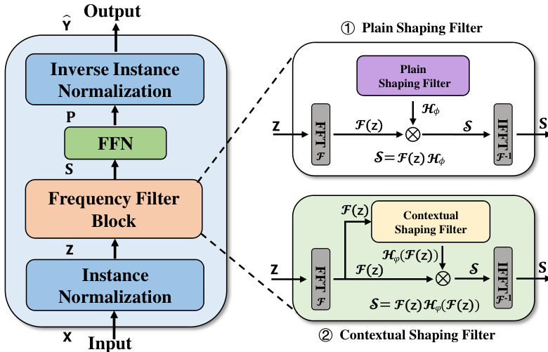
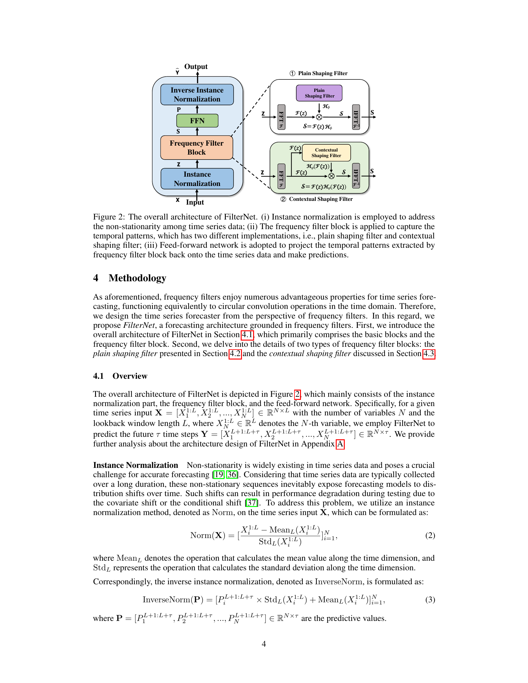
This figure illustrates the architecture of FilterNet, a time series forecasting model. The input time series data first undergoes instance normalization to handle non-stationarity. Then, a frequency filter block processes the data, choosing between a plain shaping filter (using a universal kernel) or a contextual shaping filter (with a data-dependent kernel) to extract key temporal features. Finally, a feed-forward network maps these features to produce the forecast.

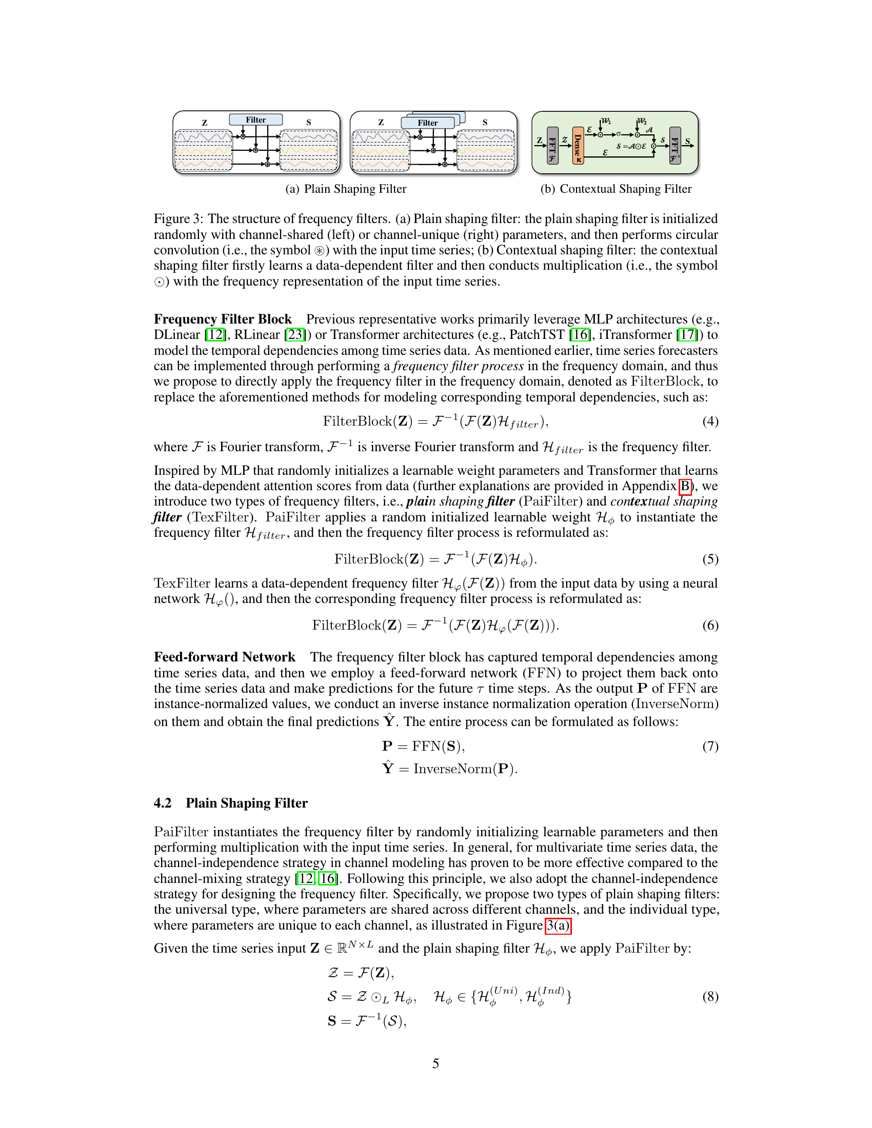
This figure shows the architecture of two types of learnable frequency filters used in the FilterNet model. The plain shaping filter uses a randomly initialized, universal frequency kernel for filtering and temporal modeling. The kernel can be either shared across channels or unique per channel. The contextual shaping filter learns a data-dependent filter to perform frequency filtering and utilizes filtered frequencies for dependency learning, thus adapting to the input signals’ characteristics. Both filter types perform a circular convolution or multiplication with the frequency representation of the input time series.

The figure demonstrates the performance of the Mean Squared Error (MSE) metric on a synthetic multi-frequency signal. It compares the performance of the iTransformer model (state-of-the-art) and FilterNet (the proposed model). The input signal consists of low, middle, and high-frequency components. FilterNet achieves significantly lower MSE (2.7e-05) compared to iTransformer (1.1e-01), indicating its superior performance in handling multi-frequency signals. This highlights FilterNet’s ability to utilize the full frequency spectrum effectively, unlike the iTransformer which struggles with high-frequency components. More detail on the experimental setup is provided in Appendix C.4 of the paper.

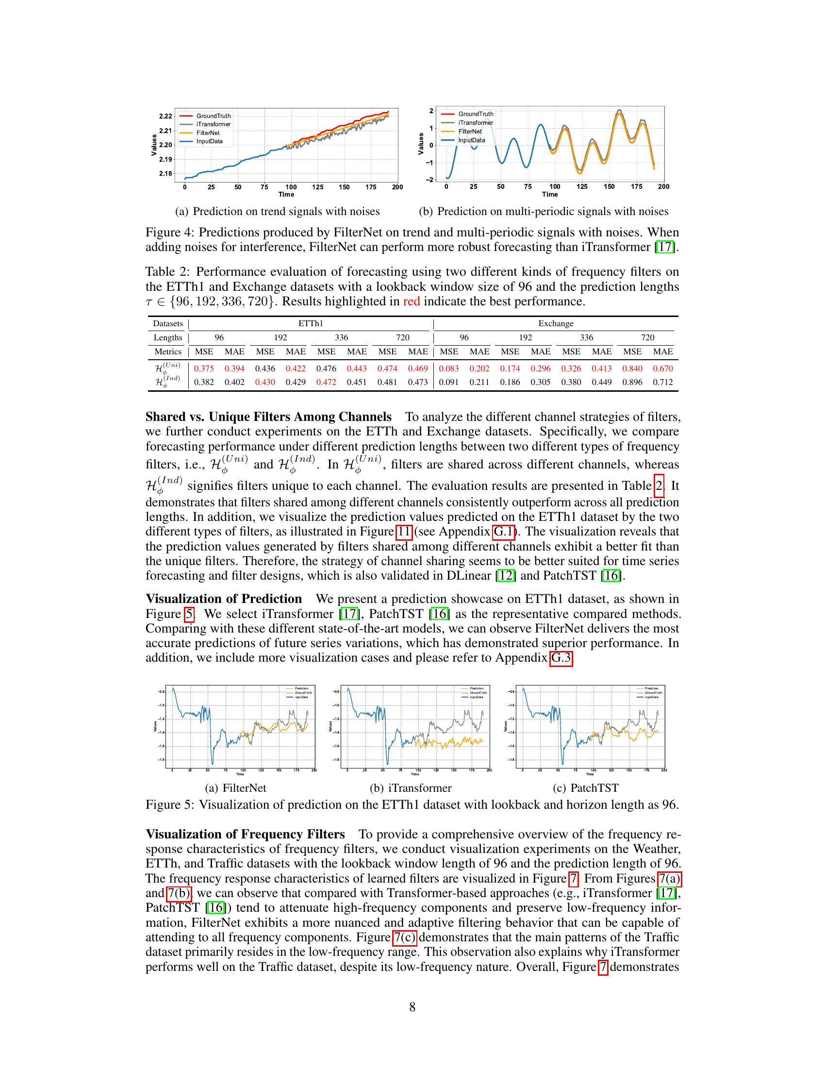
This figure visualizes the prediction results of three different models (FilterNet, iTransformer, and PatchTST) on the ETTh1 dataset. Each plot shows the ground truth, input data, and predictions. The x-axis represents the time, and the y-axis represents the values. The purpose is to provide a visual comparison of the forecasting performance of these three models. FilterNet seems to align better with the ground truth compared to iTransformer and PatchTST.

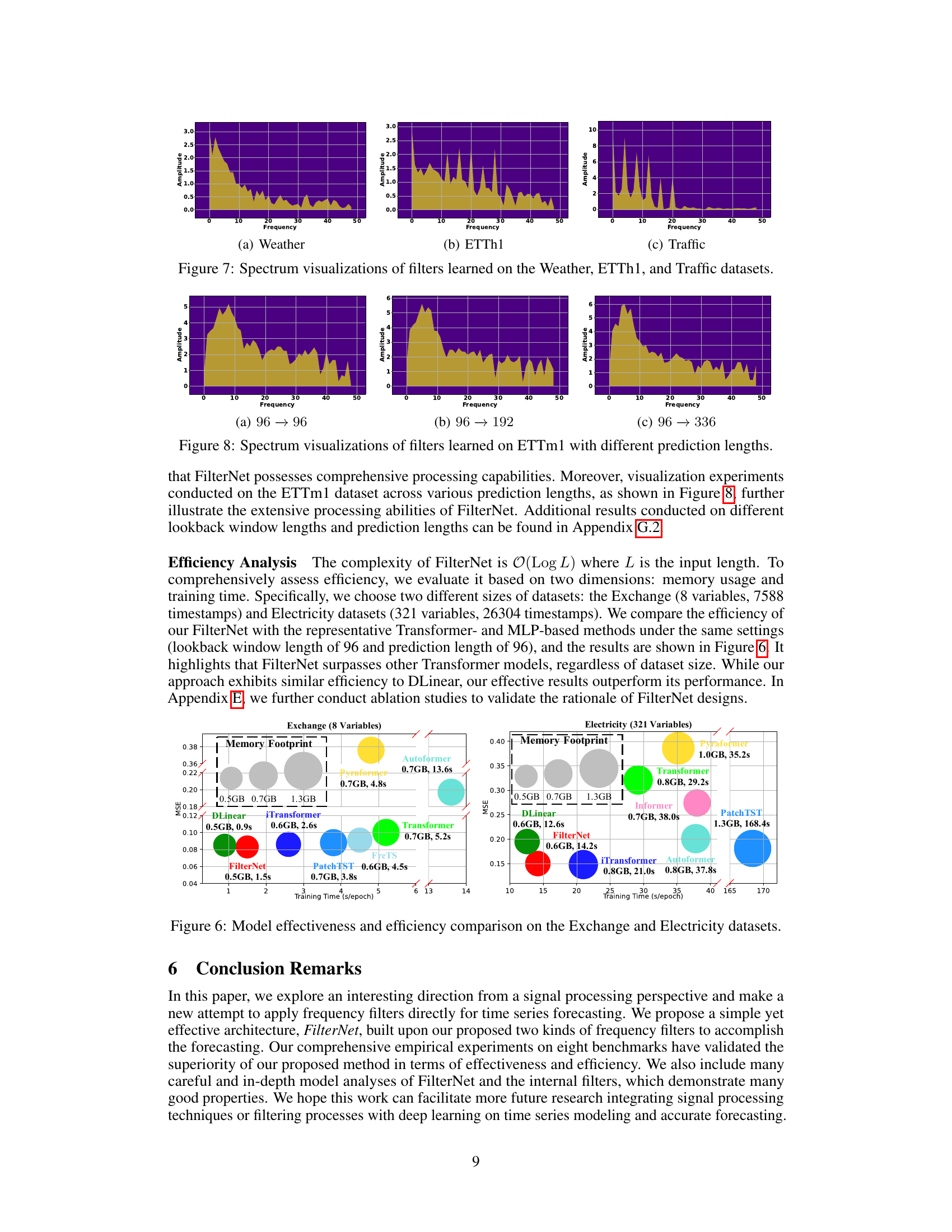
This figure visualizes the frequency response characteristics of the learned filters for three different datasets: Weather, ETTh1, and Traffic. Each subfigure shows a spectrum plot, representing the amplitude of different frequency components present in the learned filter. The x-axis represents frequency, and the y-axis represents amplitude. The plots provide insights into which frequency components are emphasized or attenuated by the filters for each dataset, revealing the filters’ selectivity in capturing relevant temporal patterns in the time series data. Differences in the spectra across datasets highlight the data-adaptive nature of the filter learning process, adjusting its frequency response based on the unique characteristics of each dataset.

This figure visualizes the frequency response characteristics of the learned filters for three different datasets: Weather, ETTh1, and Traffic. Each subfigure shows the spectrum of a filter, with the x-axis representing frequency and the y-axis representing amplitude. The visualizations help to understand how the filters selectively pass or attenuate different frequency components of the input time series data for each dataset. The variations in the spectrum across datasets illustrate that the learned filters adapt their frequency responses according to the characteristics of the respective time series data.

This figure compares the effectiveness and efficiency of FilterNet against other state-of-the-art time series forecasting models (DLinear, iTransformer, Autoformer, Pyraformer, Transformer, PatchTST, and FreTS) across two datasets: Exchange (with 8 variables) and Electricity (with 321 variables). It visualizes the memory footprint and training time (in seconds per epoch) for each model, showing FilterNet’s superior performance in terms of both efficiency and accuracy in time series forecasting. The size of the circles represents the memory footprint, while the horizontal position represents the training time. The figure effectively demonstrates the advantage of FilterNet in terms of resource utilization and speed.

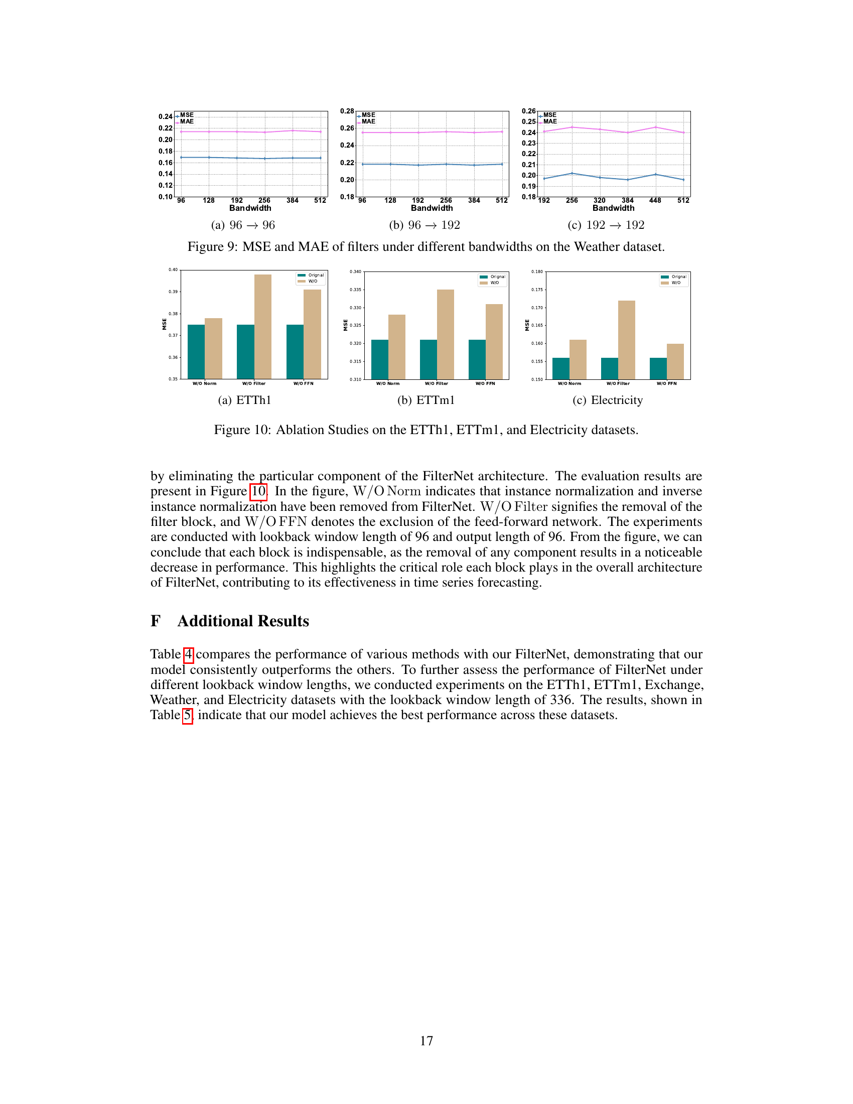
This figure visualizes the impact of different filter bandwidths on the model’s performance using the MSE (Mean Squared Error) and MAE (Mean Absolute Error) metrics for the Weather dataset. It shows three scenarios with varying lookback window lengths and prediction lengths. The results show a relationship between bandwidth and the effectiveness of the filters in making accurate predictions.

This figure shows the performance comparison between iTransformer and FilterNet on a simple synthetic multi-frequency signal. The input signal is composed of low-, middle-, and high-frequency components. The figure demonstrates that FilterNet achieves significantly lower MSE (Mean Squared Error) compared to iTransformer, highlighting FilterNet’s superior performance in handling multi-frequency signals.
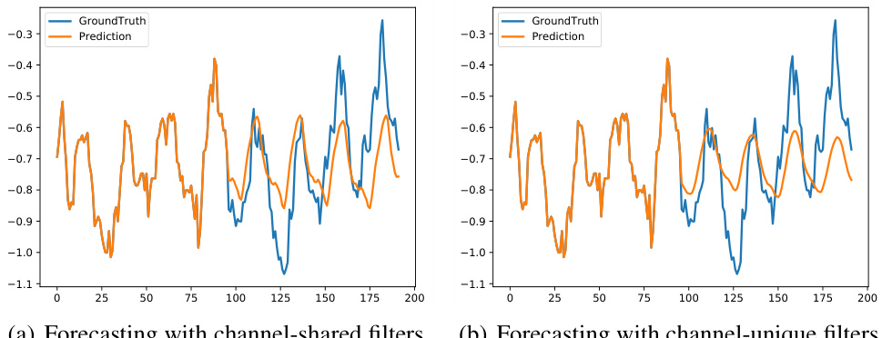
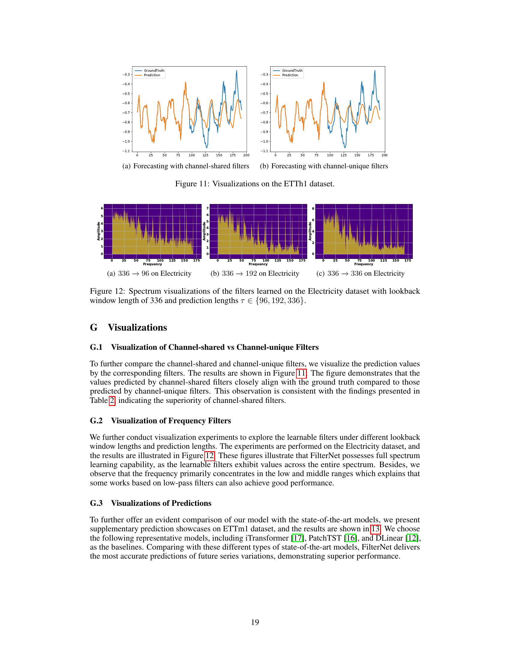
The figure compares the forecasting results of the ETTh1 dataset using channel-shared and channel-unique filters. The visualization shows that the predictions from the channel-shared filters align more closely with the ground truth compared to the channel-unique filters. This observation supports the findings in Table 2, indicating that channel-shared filters provide better forecasting performance.

This figure visualizes the frequency response characteristics of the learned filters for three different datasets: Weather, ETTh1, and Traffic. Each sub-figure shows the spectrum (amplitude vs. frequency) of a filter learned by the FilterNet model on a particular dataset. The visualizations provide insights into how the filters selectively attend to different frequency components in the input time series data. The distinct patterns in each spectrum highlight the dataset-specific frequency characteristics captured by the filters, demonstrating the filter’s ability to adapt to the unique properties of various time series.
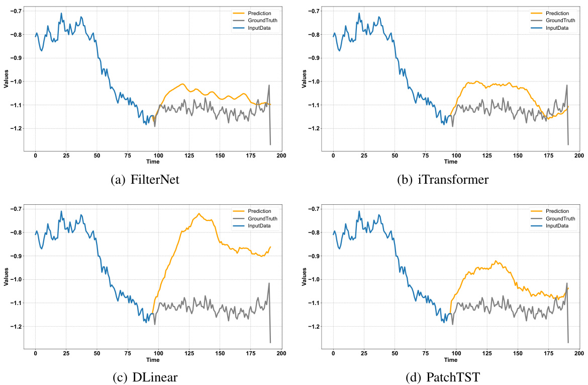
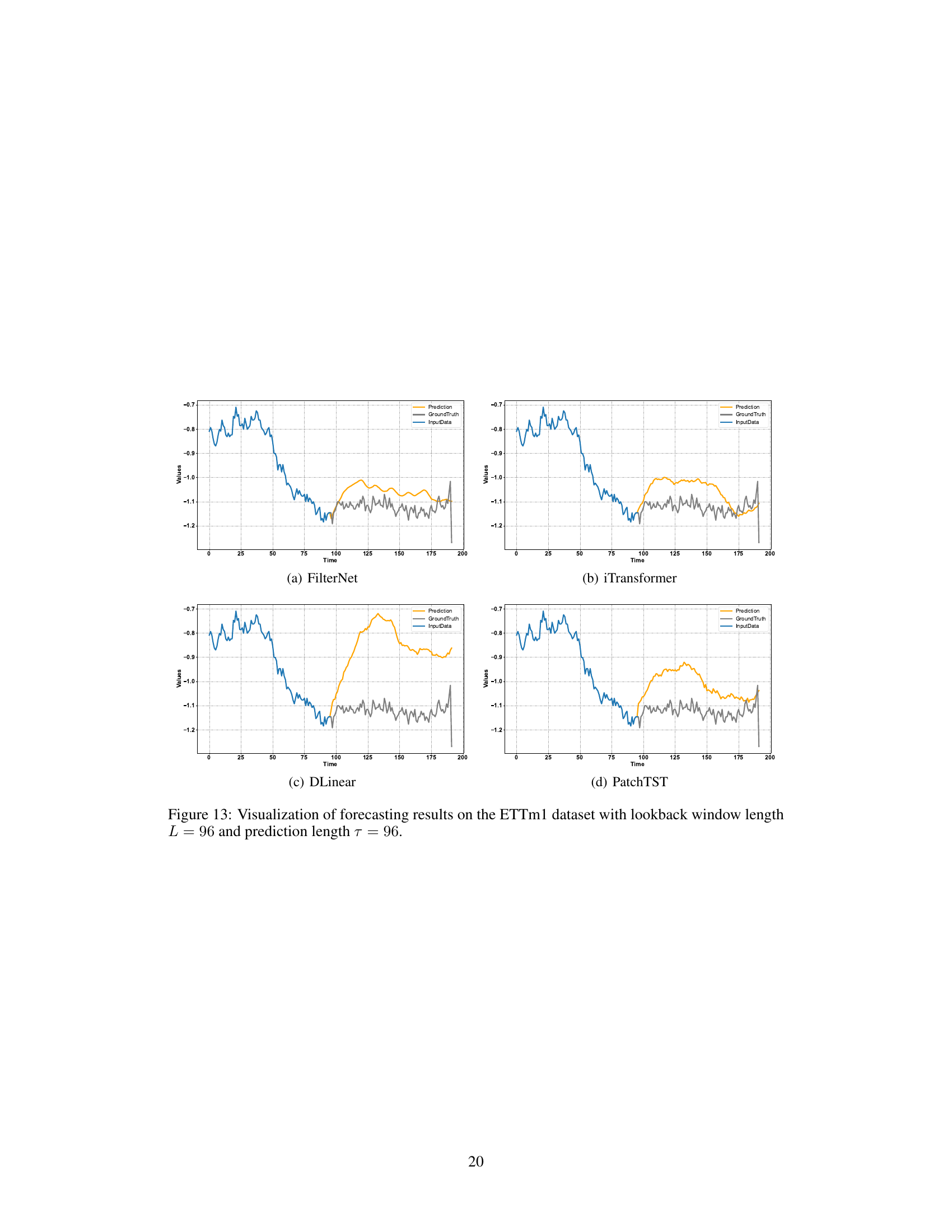
This figure visualizes the prediction results of FilterNet, iTransformer, and PatchTST on the ETTh1 dataset. The lookback and horizon lengths are both set to 96. The figure shows that FilterNet achieves better prediction accuracy compared to the other two models, indicating its superior performance in time series forecasting.
More on tables

This table presents the performance comparison of using two types of frequency filters (channel-shared and channel-unique) in FilterNet for time series forecasting. The comparison is made on two benchmark datasets, ETTh1 and Exchange, across four different prediction lengths (96, 192, 336, and 720 time steps). The lookback window length is kept constant at 96. The metrics used for evaluation are MSE (Mean Squared Error) and MAE (Mean Absolute Error). The best-performing filter type for each dataset and prediction length is highlighted in red.

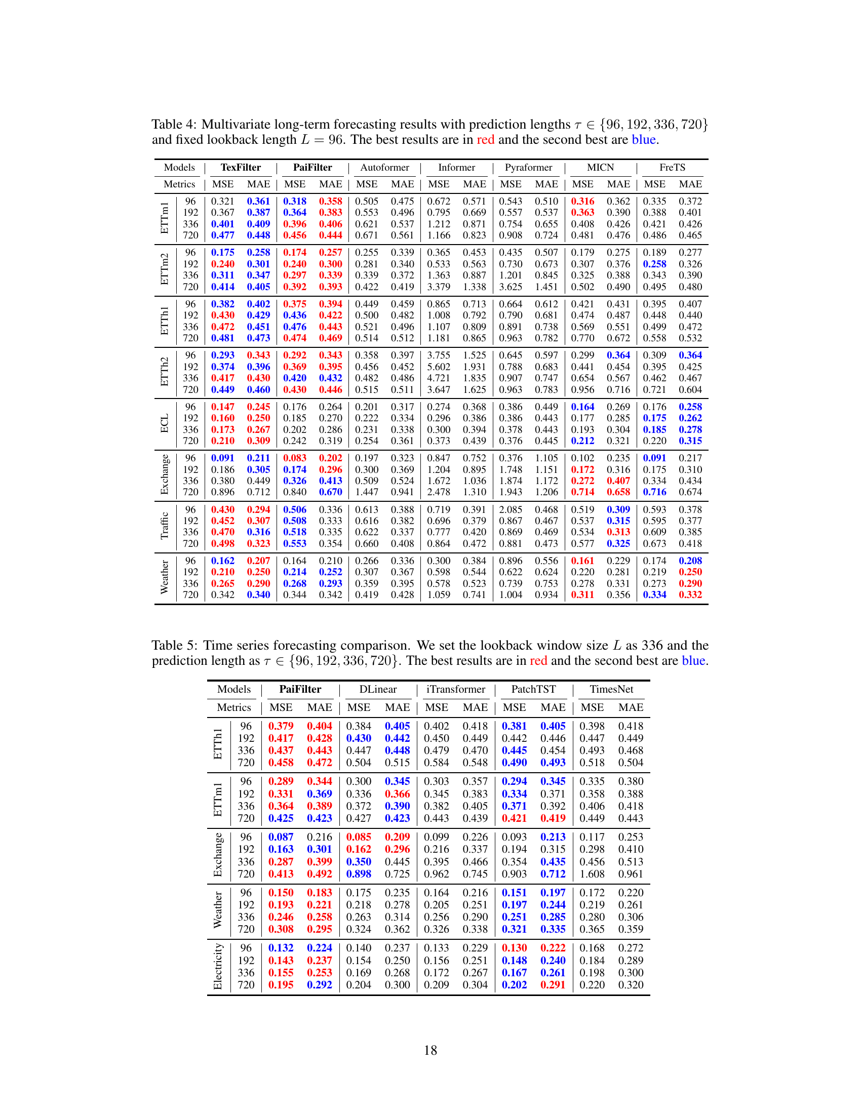
This table presents the forecasting results for various prediction lengths (96, 192, 336, and 720 time steps) using a lookback window of 96 time steps. It compares the performance of FilterNet (with both plain and contextual shaping filters) against several other state-of-the-art time series forecasting models across eight benchmark datasets (ETTm1, ETTm2, ETTh1, ETTh2, Weather, Traffic, Exchange, and Electricity). The best performing model for each metric and dataset is highlighted in red, while the second best is in blue. Due to space constraints, additional results using other baselines and different lookback window lengths are provided in Tables 4 and 5 in the paper’s appendix.
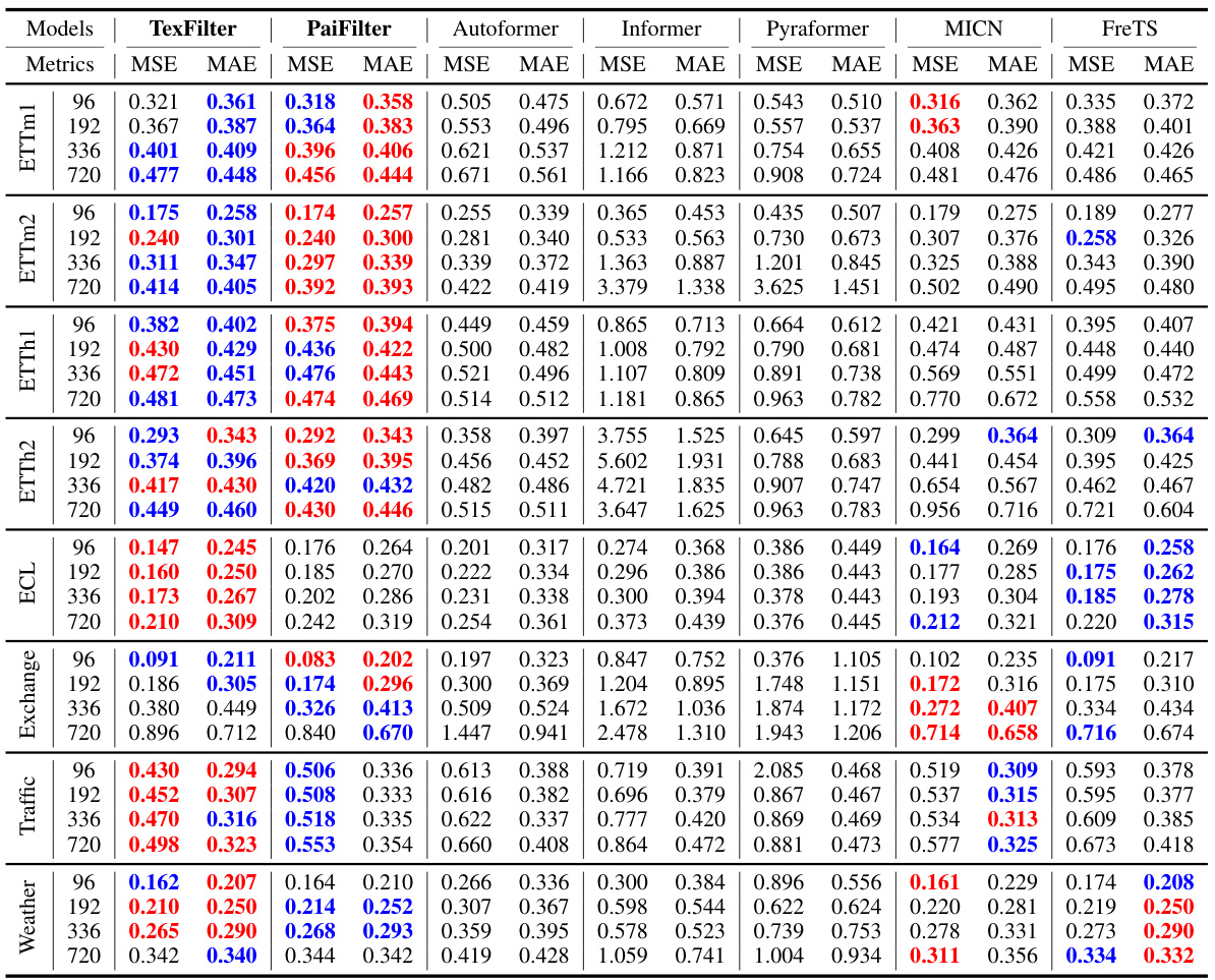
This table presents the Mean Squared Error (MSE) and Mean Absolute Error (MAE) for various time series forecasting models on eight benchmark datasets. Different prediction lengths (τ) are tested, while keeping the lookback window length (L) constant at 96. The best and second-best performing models for each dataset and prediction length are highlighted in red and blue respectively. Due to space constraints, additional results using different lookback lengths and other benchmark models are provided in Tables 4 and 5 within the paper.
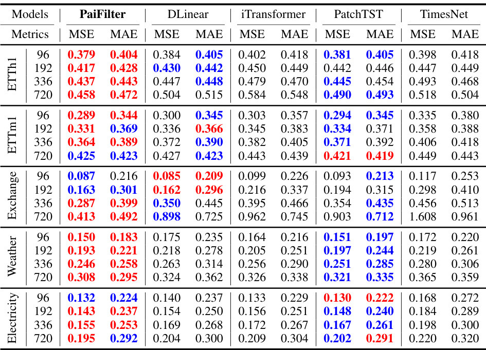
This table presents the forecasting performance of FilterNet and several other state-of-the-art time series forecasting models on eight benchmark datasets. For each dataset and prediction length, it shows the Mean Squared Error (MSE) and Mean Absolute Error (MAE) achieved by each model. The best performing model for each metric is highlighted in red and the second best in blue. The table focuses on a lookback window length of 96, with additional results for other lengths provided in supplementary tables.
Full paper#
