TL;DR#
Tree ensembles, popular machine learning models, are vulnerable to adversarial attacks—slightly altered inputs that cause misclassifications. Existing methods for generating these adversarial examples are computationally expensive, especially when dealing with large datasets, as they treat each example independently. This is inefficient because regularities exist across the generated examples.
This paper introduces a novel method to overcome this inefficiency. It leverages the observation that adversarial examples commonly perturb the same set of features. By identifying these features, the researchers develop two algorithms that significantly accelerate the process. Their approach demonstrates substantial speed improvements, making the generation of adversarial examples faster and more scalable.
Key Takeaways#
Why does it matter?#
This paper is crucial for researchers working on adversarial machine learning and tree ensemble models. It offers a novel approach to significantly speed up the process of generating adversarial examples, which is essential for various tasks such as model evaluation, robustness checking, and attack generation. The proposed method is theoretically grounded and empirically validated, paving the way for more efficient and scalable adversarial attacks and defenses.
Visual Insights#

🔼 This figure shows the distribution of modified attributes in adversarial examples generated for the mnist and webspam datasets using the kantchelian approach. The x-axis categorizes attributes based on the frequency of their modification (never, less than 5%, or greater than or equal to 5%). The y-axis represents the number of attributes falling into each category. The results highlight that a relatively small set of attributes are consistently perturbed to generate adversarial examples, suggesting an opportunity for optimization.
read the caption
Figure 1: Bar plots showing that most attributes are not modified by the majority of adversarial examples on the mnist and webspam datasets. The leftmost bar shows the number of attributes that are never changed by any of the 10000 adversarial examples generated by kantchelian's approach. The middle bar shows the number of attributes that are modified at least once but at most by 5% of the adversarial examples. The rightmost bar shows the number of frequently modified features.
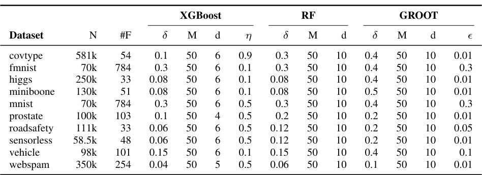
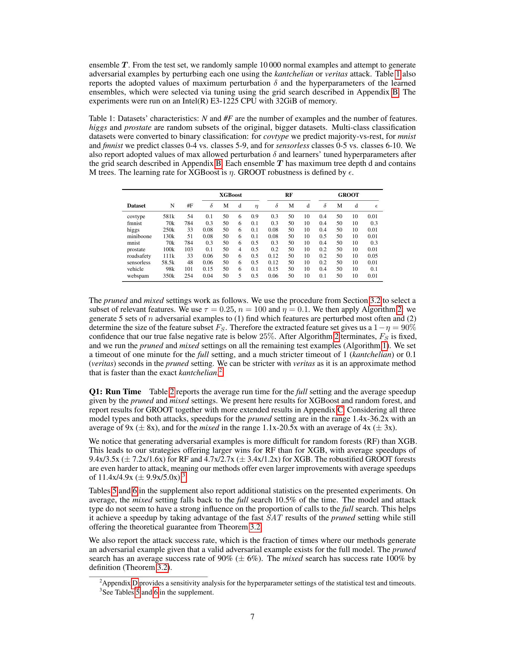
🔼 This table presents the characteristics of the ten datasets used in the experiments. For each dataset, it shows the number of examples (N), number of features (#F), the maximum perturbation size (δ) used, and hyperparameters for three different ensemble models (XGBoost, Random Forest, GROOT): the number of trees (M), maximum tree depth (d), learning rate (η for XGBoost), and robustness parameter (ε for GROOT). It also notes that multi-class datasets were converted to binary classification problems, specifying how this conversion was done.
read the caption
Table 1: Datasets' characteristics: N and #F are the number of examples and the number of features. higgs and prostate are random subsets of the original, bigger datasets. Multi-class classification datasets were converted to binary classification: for covtype we predict majority-vs-rest, for mnist and fmnist we predict classes 0-4 vs. classes 5-9, and for sensorless classes 0-5 vs. classes 6-10. We also report adopted values of max allowed perturbation δ and learners' tuned hyperparameters after the grid search described in Appendix B. Each ensemble T has maximum tree depth d and contains M trees. The learning rate for XGBoost is η. GROOT robustness is defined by ε.
In-depth insights#
Adversarial Attacks#
Adversarial attacks are a critical concern in machine learning, particularly for tree ensembles. These attacks involve creating slightly perturbed inputs that cause a model to misclassify, essentially fooling it. The core challenge lies in the computational cost of generating these adversarial examples, especially when dealing with large datasets or complex models. Current methods often require solving the problem from scratch for each data point, leading to inefficiency. However, a key insight is that adversarial examples for a given model tend to perturb a consistent, small set of features. This observation allows for improvements; by identifying this set, the search space for generating attacks can be significantly reduced. This is a novel approach that exploits regularities across multiple similar problems. Two strategies are proposed: one theoretically grounded, and another that guarantees a solution if one exists. These methods can greatly improve the efficiency of generating adversarial examples, leading to substantial speedups. This is valuable not just for understanding model vulnerabilities, but also for applications like security testing and improving model robustness.
Ensemble Pruning#
Ensemble pruning, a crucial technique in machine learning, aims to improve model efficiency and performance by strategically removing less-important trees or components from an ensemble. It addresses the challenge of ensembles, which can be computationally expensive and prone to overfitting. Thoughtful pruning techniques must balance reducing complexity with maintaining accuracy. Several approaches exist, including those based on tree-specific metrics (e.g., impurity, depth), global performance evaluation (e.g., cross-validation, held-out data), or a combination. The optimal pruning strategy often depends on the ensemble type, the dataset, and the desired trade-off between model size and predictive power. Careful consideration of bias and variance is key, as poorly implemented pruning can increase prediction error. Advanced techniques incorporate feature importance analysis or explore alternative tree structures to optimize the pruning process. Ultimately, effective ensemble pruning is a powerful tool for creating more robust, interpretable, and efficient models within machine learning.
Feature Subset#
The concept of a ‘Feature Subset’ in machine learning, particularly within the context of adversarial example generation for tree ensembles, is crucial for efficiency. Selecting a relevant subset of features to perturb allows for a significant reduction in the search space, drastically decreasing the computational cost of finding adversarial examples. The effectiveness hinges on the hypothesis that adversarial examples primarily manipulate a small, consistent set of features across multiple similar instances. Identifying this key subset requires careful analysis of previously generated adversarial examples, potentially employing statistical methods to discern frequently perturbed features from less influential ones. This process creates a pruned or modified version of the original ensemble model, which then forms the basis for generating new adversarial examples more efficiently. The trade-off lies in balancing speed improvements with the risk of introducing false negatives; a smaller subset leads to faster computations but might miss adversarial examples that rely on features outside the subset. Therefore, a well-defined strategy to select the feature subset is essential to optimize both speed and accuracy.
Empirical Results#
An Empirical Results section in a research paper would typically present quantitative findings that validate the study’s hypotheses or address its research questions. A strong Empirical Results section would begin by clearly stating the metrics used to evaluate the study’s claims. It should then present the results in a clear, concise manner, often using tables and figures to effectively communicate complex data. Visualizations are key to easily communicating the main findings, particularly if dealing with many variables. Statistical significance should be explicitly addressed; p-values, confidence intervals, or effect sizes would be reported along with appropriate discussion. Importantly, any limitations of the analysis method or unexpected results should be transparently acknowledged. The results’ interpretation should focus on their implications for the overarching research goals, connecting them back to the paper’s central arguments. The section should conclude with a summary of the key findings, highlighting their significance and impact within the broader research context.
Future Work#
The paper’s omission of a ‘Future Work’ section is notable. A dedicated section would ideally explore avenues for improving the proposed method. This could involve investigating alternative feature selection techniques beyond the statistical test used, potentially incorporating domain expertise or feature importance scores from the base models. Another promising direction would be to assess the impact of varying timeout values used for the pruned approach. Experimentation with a wider range of timeout values could reveal an optimal trade-off between speed and accuracy. Furthermore, a more in-depth analysis of the false negative rates and its impact on different dataset characteristics would be useful. Finally, exploring the applicability of the technique to other model classes beyond tree ensembles is a key area for future development, as this could greatly expand the practical impact and generalizability of the findings.
More visual insights#
More on figures

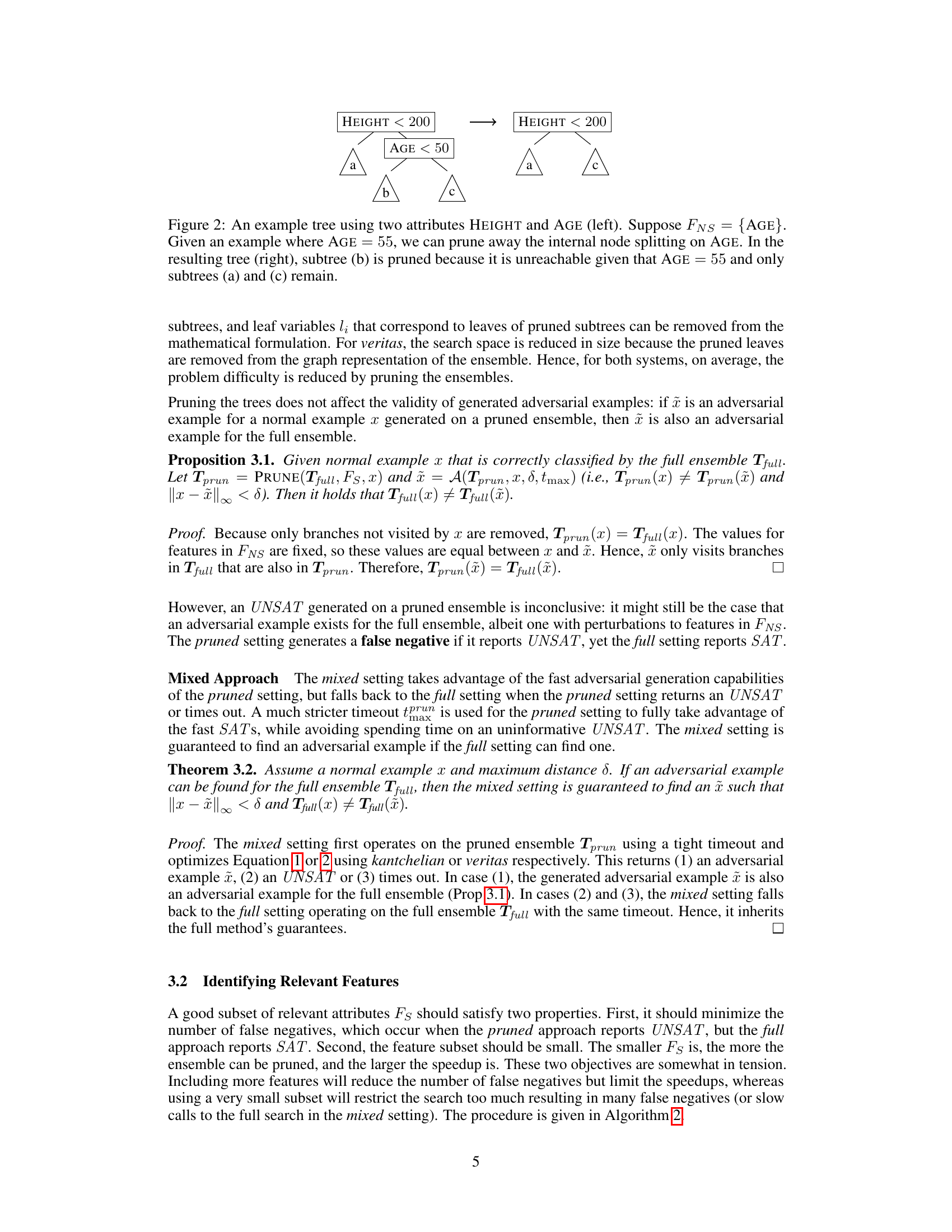
🔼 This figure illustrates the pruning process in the paper’s proposed approach. The left side shows a tree with two attributes, HEIGHT and AGE, where AGE is a split condition below a HEIGHT split. The right side demonstrates the pruning of the subtree (b) under the condition that the AGE attribute is fixed to a value (55) that is greater than the split threshold (50). This pruning is based on the fact that the path to subtree (b) is now unreachable given the fixed value of AGE. The result is a simplified tree that is more computationally efficient for the algorithms that generate adversarial examples.
read the caption
Figure 2: An example tree using two attributes HEIGHT and AGE (left). Suppose FNS = {AGE}. Given an example where AGE = 55, we can prune away the internal node splitting on AGE. In the resulting tree (right), subtree (b) is pruned because it is unreachable given that AGE = 55 and only subtrees (a) and (c) remain.
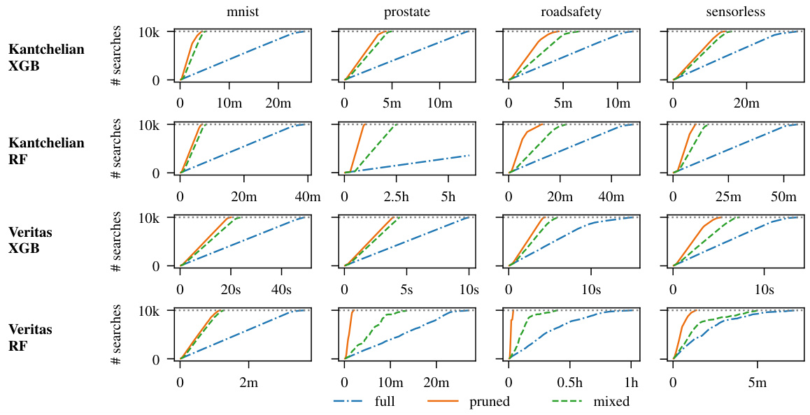
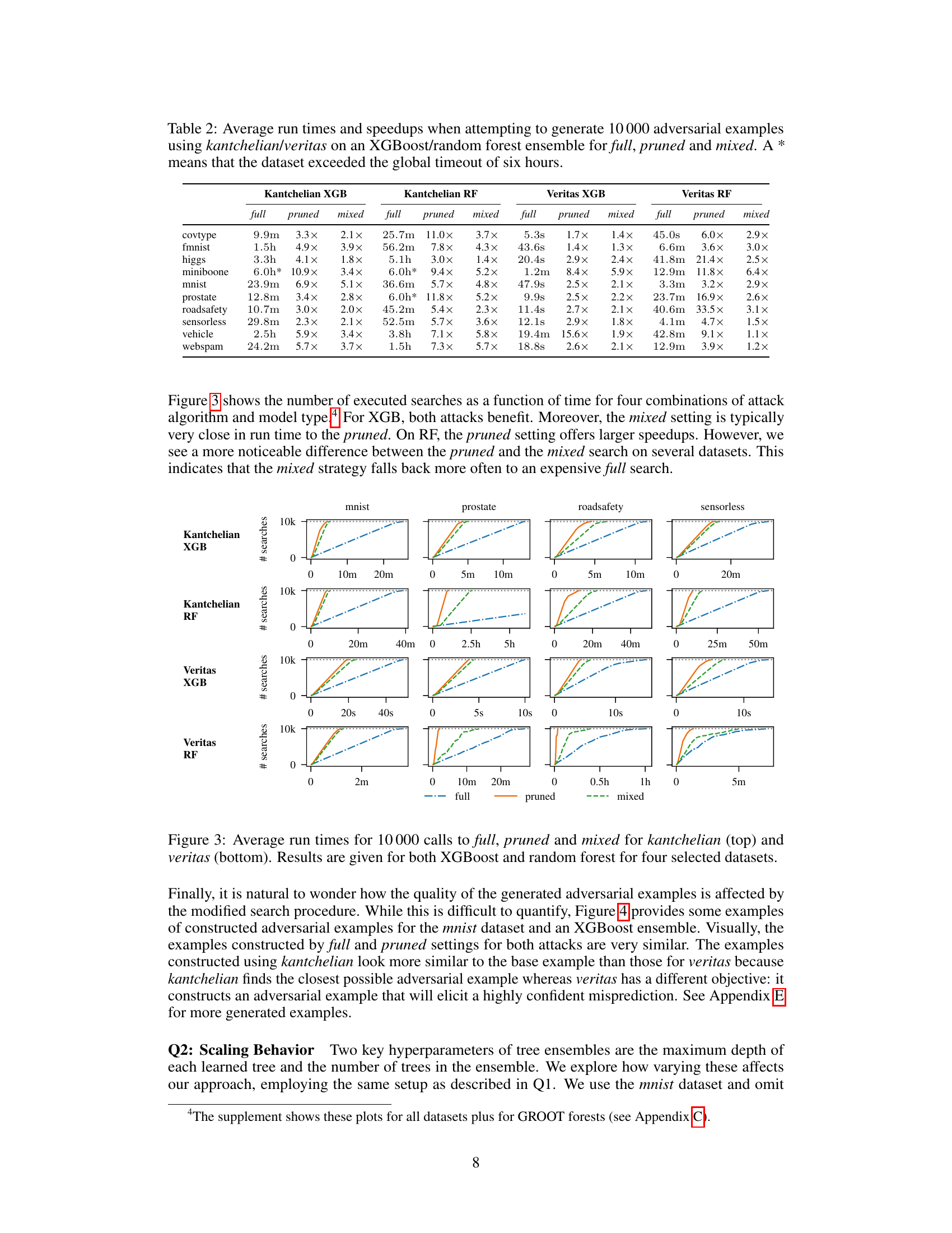
🔼 This figure compares the run times of three adversarial example generation methods: full, pruned, and mixed. The methods are applied using two different algorithms (kantchelian and veritas) for both XGBoost and random forest models. The results are shown for four representative datasets (mnist, prostate, roadsafety, sensorless). The figure visually demonstrates the significant speedup achieved by the pruned and mixed methods, especially compared to the original full search approach.
read the caption
Figure 3: Average run times for 10000 calls to full, pruned and mixed for kantchelian (top) and veritas (bottom). Results are given for both XGBoost and random forest for four selected datasets.

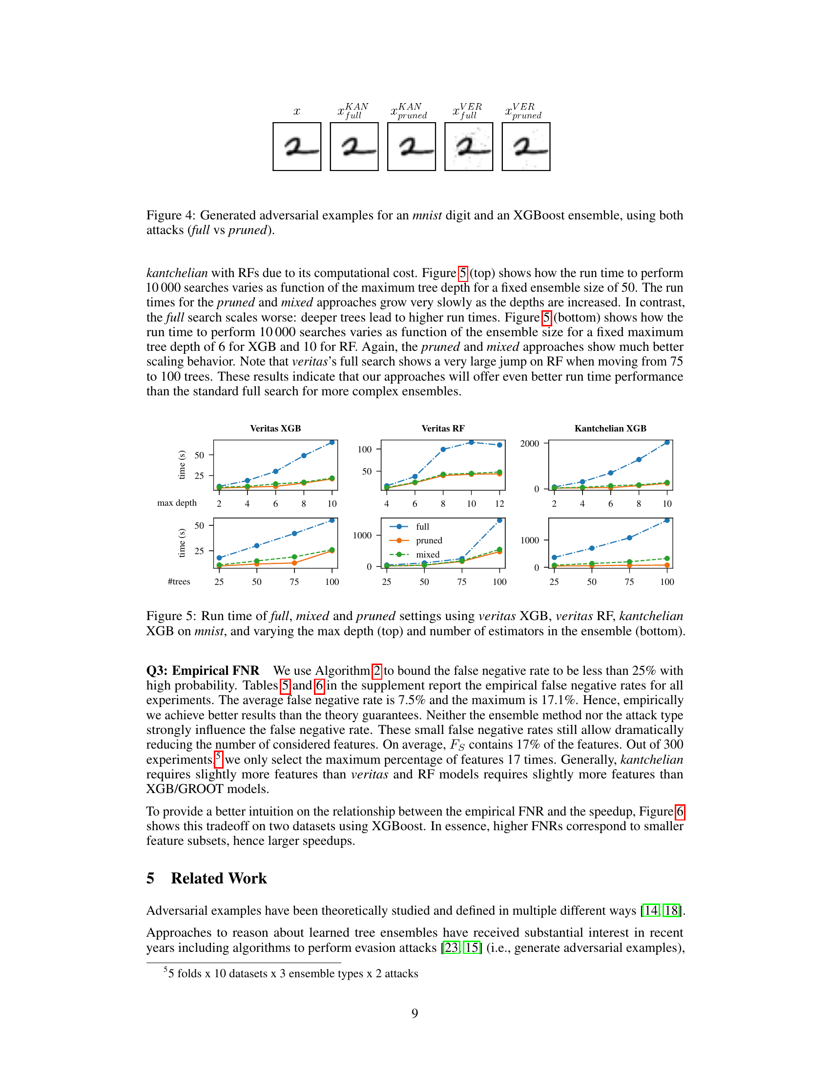
🔼 This figure displays adversarial examples generated for a handwritten digit ‘2’ from the MNIST dataset using two different attack methods: Kantchelian and Veritas. Each attack method is shown with two variants: the ‘full’ version where all features can be modified, and a ‘pruned’ version where only a subset of features determined to be most frequently perturbed are modified. The goal is to show that using a pruned set of features does not significantly impact the quality of the adversarial examples generated, while drastically reducing the computation time.
read the caption
Figure 4: Generated adversarial examples for an mnist digit and an XGBoost ensemble, using both attacks (full vs pruned).

🔼 This figure shows how the run time to perform 10000 adversarial example generation searches varies as a function of the maximum tree depth (top) and the number of trees in the ensemble (bottom). The results are shown for three settings: full, pruned, and mixed. The full setting represents the original approach; the pruned setting only allows modifications to a subset of frequently perturbed features; and the mixed setting combines the pruned and full settings. The figure shows that the pruned and mixed approaches exhibit much better scaling behavior than the full search, particularly as the complexity of the ensemble increases.
read the caption
Figure 5: Run time of full, mixed and pruned settings using veritas XGB, veritas RF, kantchelian XGB on mnist, and varying the max depth (top) and number of estimators in the ensemble (bottom).

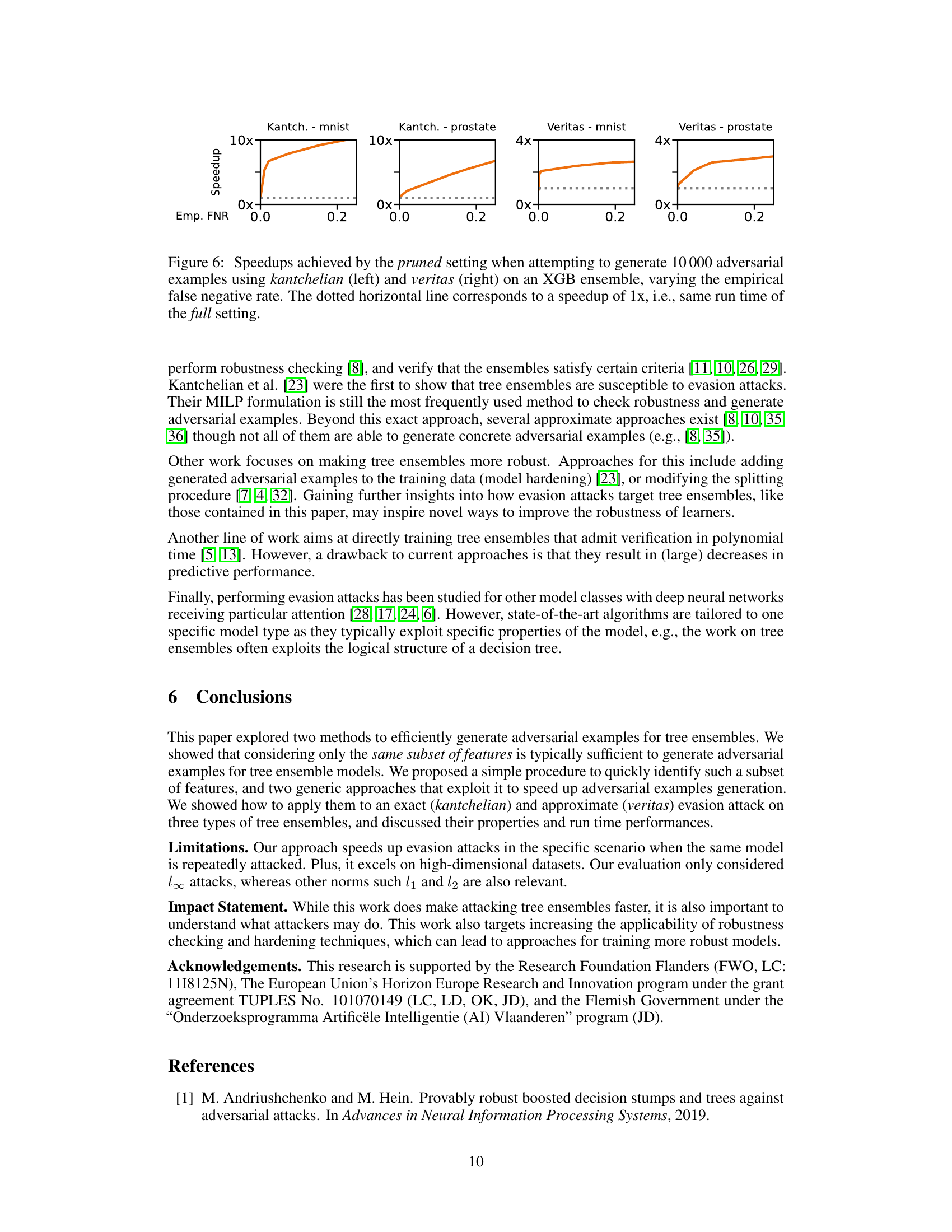
🔼 This figure shows the relationship between the empirical false negative rate (FNR) and speedup achieved by using the pruned approach for generating adversarial examples. The empirical FNR is the percentage of times where the pruned approach fails to find an adversarial example while the full approach succeeds. The x-axis represents the empirical FNR, and the y-axis represents the speedup. The dotted line indicates the speedup is equal to 1, which means there is no speedup using the pruned method. The figure shows that as the FNR increases, the speedup also increases. This is because a higher FNR corresponds to smaller feature subsets, leading to a faster pruned search, even though there is a trade-off because a smaller feature subset can result in more false negatives.
read the caption
Figure 6: Speedups achieved by the pruned setting when attempting to generate 10000 adversarial examples using kantchelian (left) and veritas (right) on an XGB ensemble, varying the empirical false negative rate. The dotted horizontal line corresponds to a speedup of 1x, i.e., same run time of the full setting.

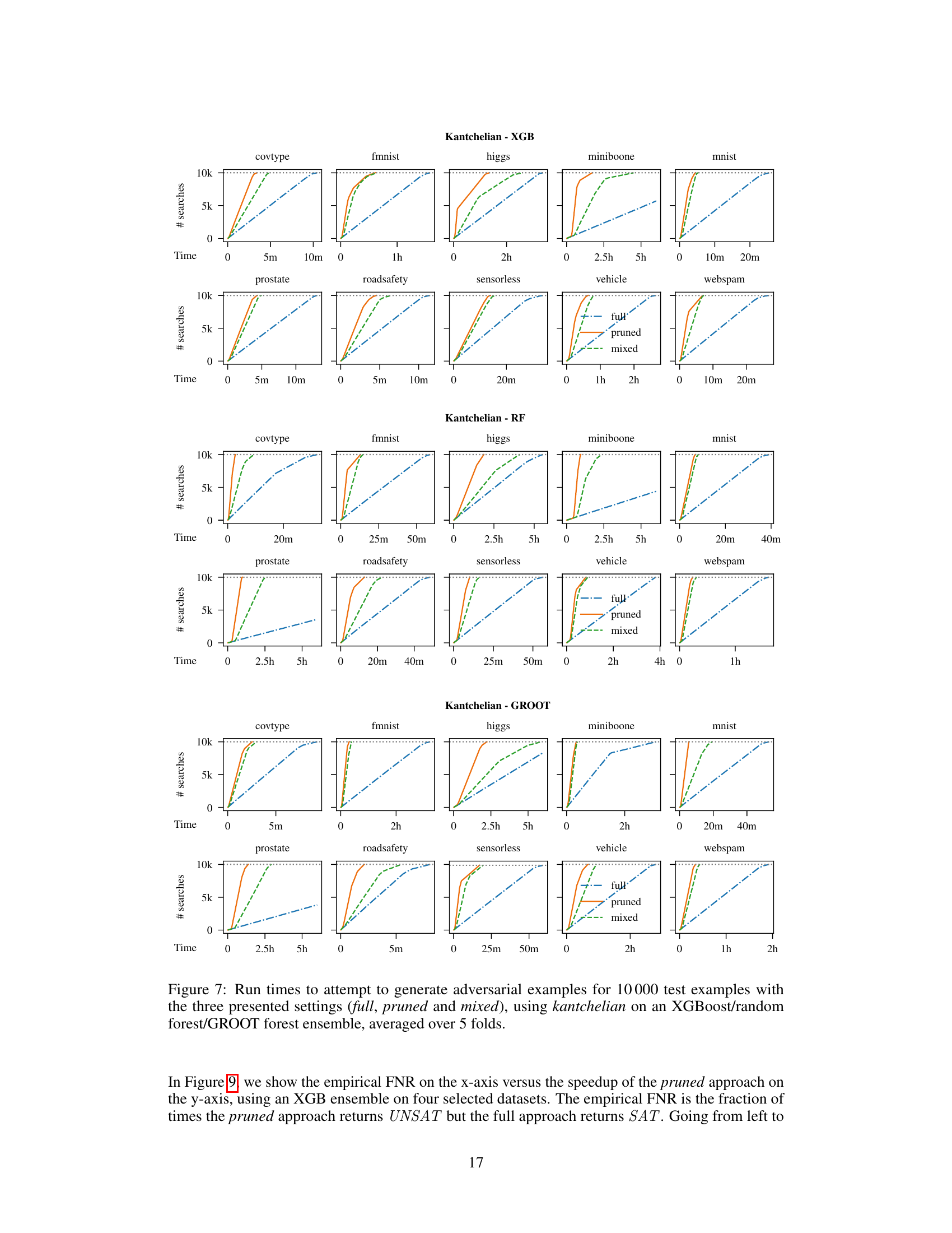
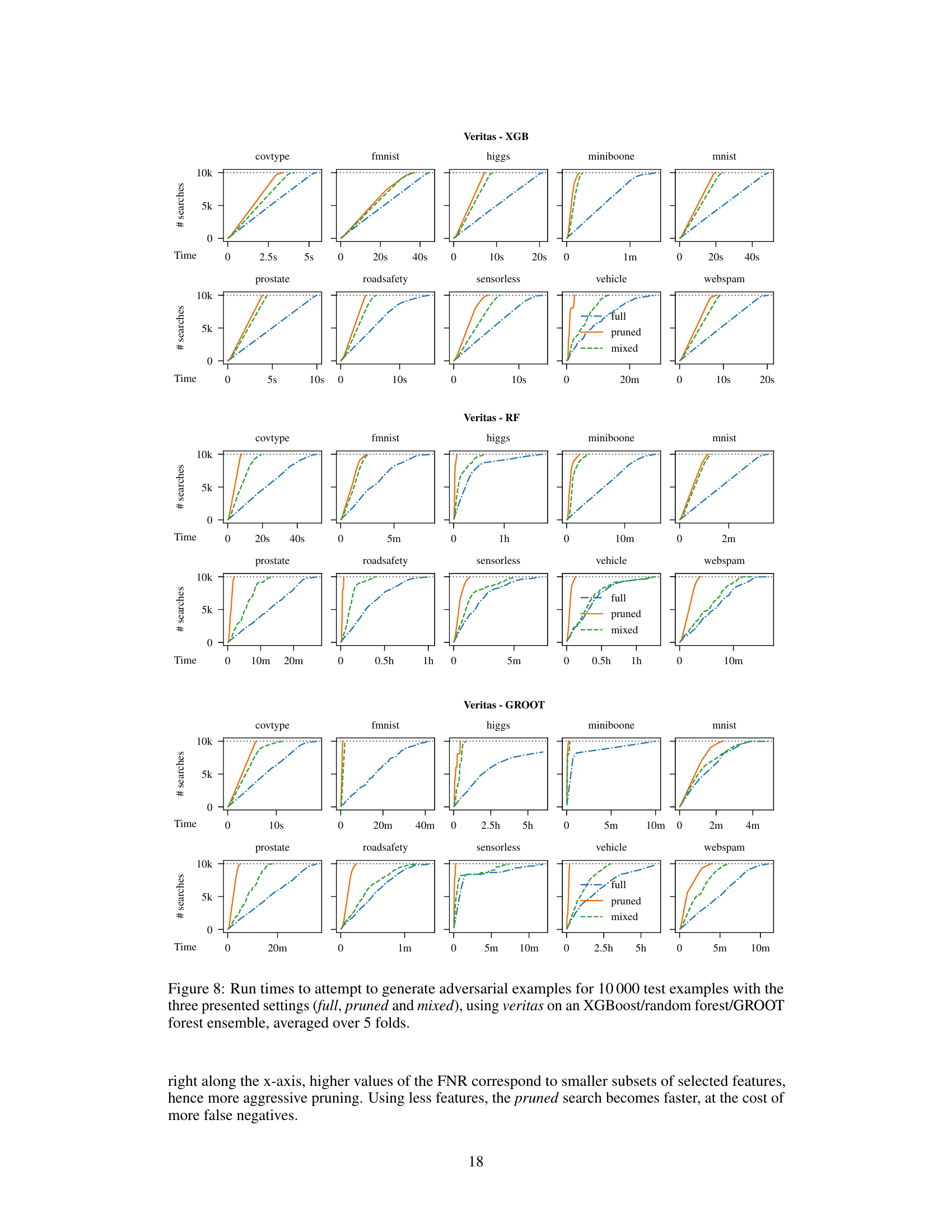
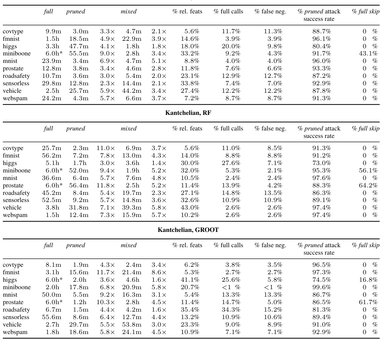
🔼 This figure shows the run time performance comparison of three adversarial example generation methods: full, pruned, and mixed. The experiment involves generating 10,000 adversarial examples using the Kantchelian method on three types of tree ensembles: XGBoost, Random Forest, and GROOT. The figure presents results averaged over 5 folds of cross-validation for 10 datasets. Each subplot represents a single dataset and shows how the number of searches (y-axis) increases over time (x-axis) for each of the three methods. The pruned and mixed methods aim to improve performance by limiting perturbations to a subset of features, which explains their faster convergence in most cases when compared to the full approach which explores the complete feature space.
read the caption
Figure 7: Run times to attempt to generate adversarial examples for 10000 test examples with the three presented settings (full, pruned and mixed), using kantchelian on an XGBoost/random forest/GROOT forest ensemble, averaged over 5 folds.

🔼 This figure shows the run time performance of three different approaches (full, pruned, and mixed) for generating adversarial examples using two different attack methods (kantchelian and veritas) on two different types of tree ensembles (XGBoost and random forest). The results are displayed for four selected datasets (mnist, prostate, roadsafety, and sensorless). It demonstrates the efficiency gains achieved by the pruned and mixed approaches in comparison to the standard full approach.
read the caption
Figure 3: Average run times for 10000 calls to full, pruned and mixed for kantchelian (top) and veritas (bottom). Results are given for both XGBoost and random forest for four selected datasets.
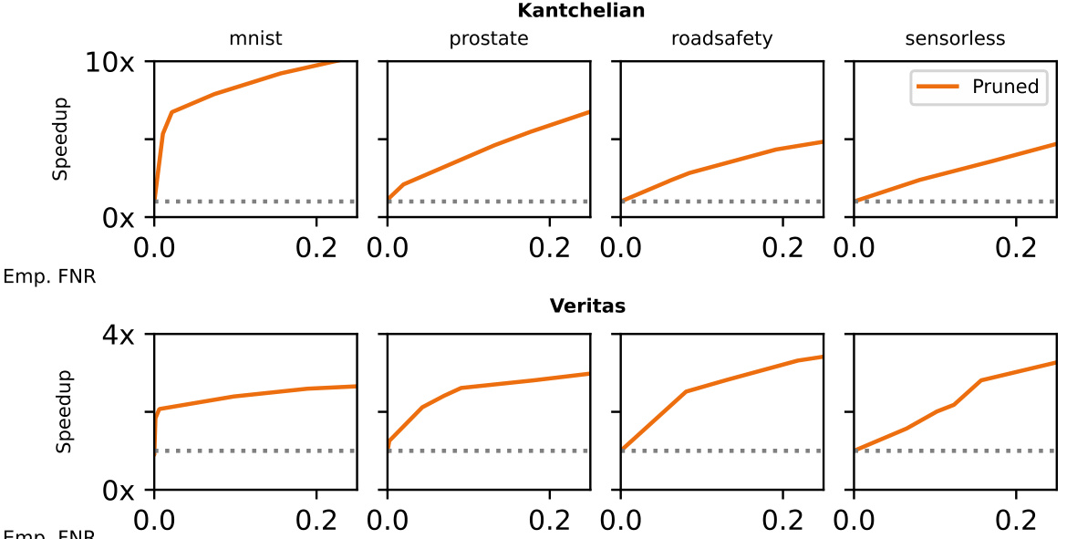
🔼 The figure shows the relationship between empirical false negative rate and speedup for the pruned setting in the context of adversarial example generation. It displays four separate plots, two for each evasion attack (Kantchelian and Veritas). Each plot shows the relationship for a different dataset (mnist, prostate, roadsafety, sensorless) and uses XGBoost. The speedup is the run time of the full approach relative to that of the pruned approach, with the empirical false negative rate being the fraction of times the pruned search reported UNSAT while the full search reported SAT. Higher FNR generally indicates greater speedup because it implies the pruning removed many less important attributes that reduced search space without significantly harming the attack’s accuracy. The dotted line at 1x speedup represents the baseline (no speedup).
read the caption
Figure 6: Speedups achieved by the pruned setting when attempting to generate 10000 adversarial examples using kantchelian (left) and veritas (right) on an XGB ensemble, varying the empirical false negative rate. The dotted horizontal line corresponds to a speedup of 1x, i.e., same run time of the full setting.
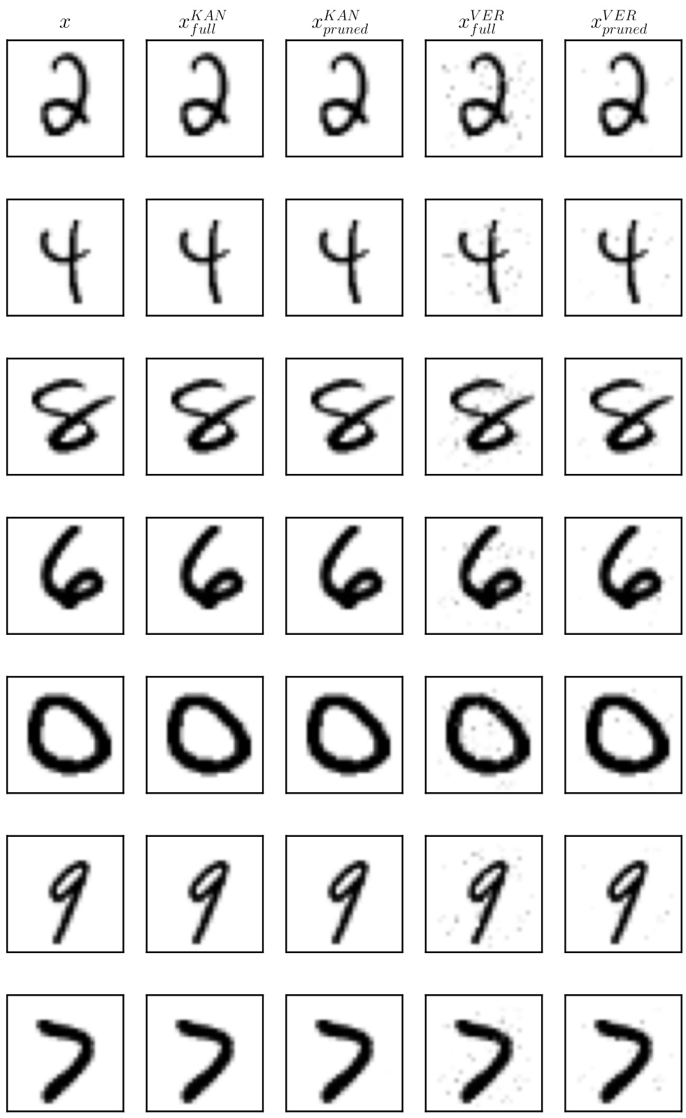
🔼 This figure shows adversarial examples generated for MNIST digits using both the Kantchelian and Veritas attacks, comparing the results obtained when using the full method (allowing modifications to all features) against the pruned method (restricting modifications to a subset of frequently perturbed features). The goal is to visually demonstrate the similarity of adversarial examples generated by both methods, supporting the claim that the pruned approach effectively generates similar adversarial examples more quickly.
read the caption
Figure 4: Generated adversarial examples for an mnist digit and an XGBoost ensemble, using both attacks (full vs pruned).
More on tables

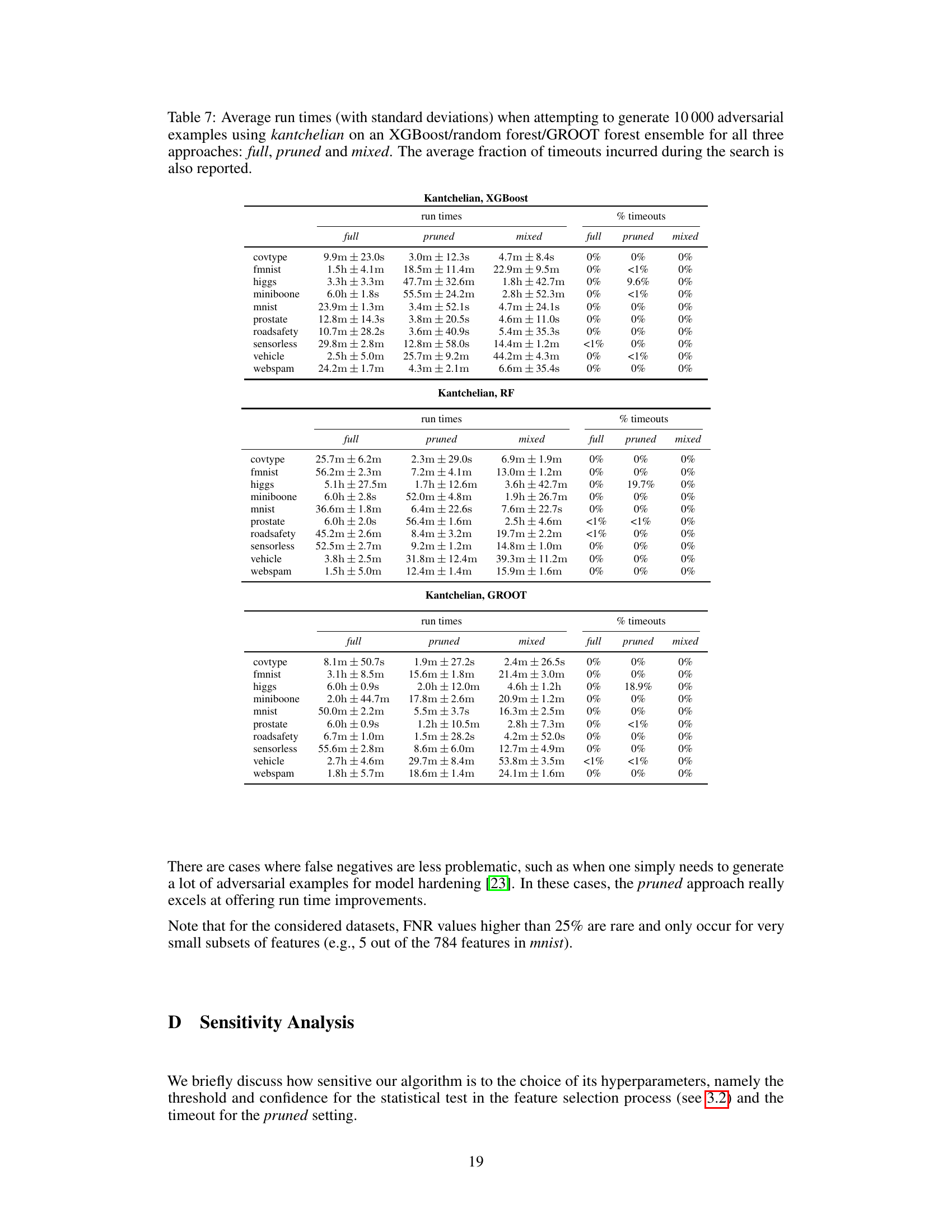
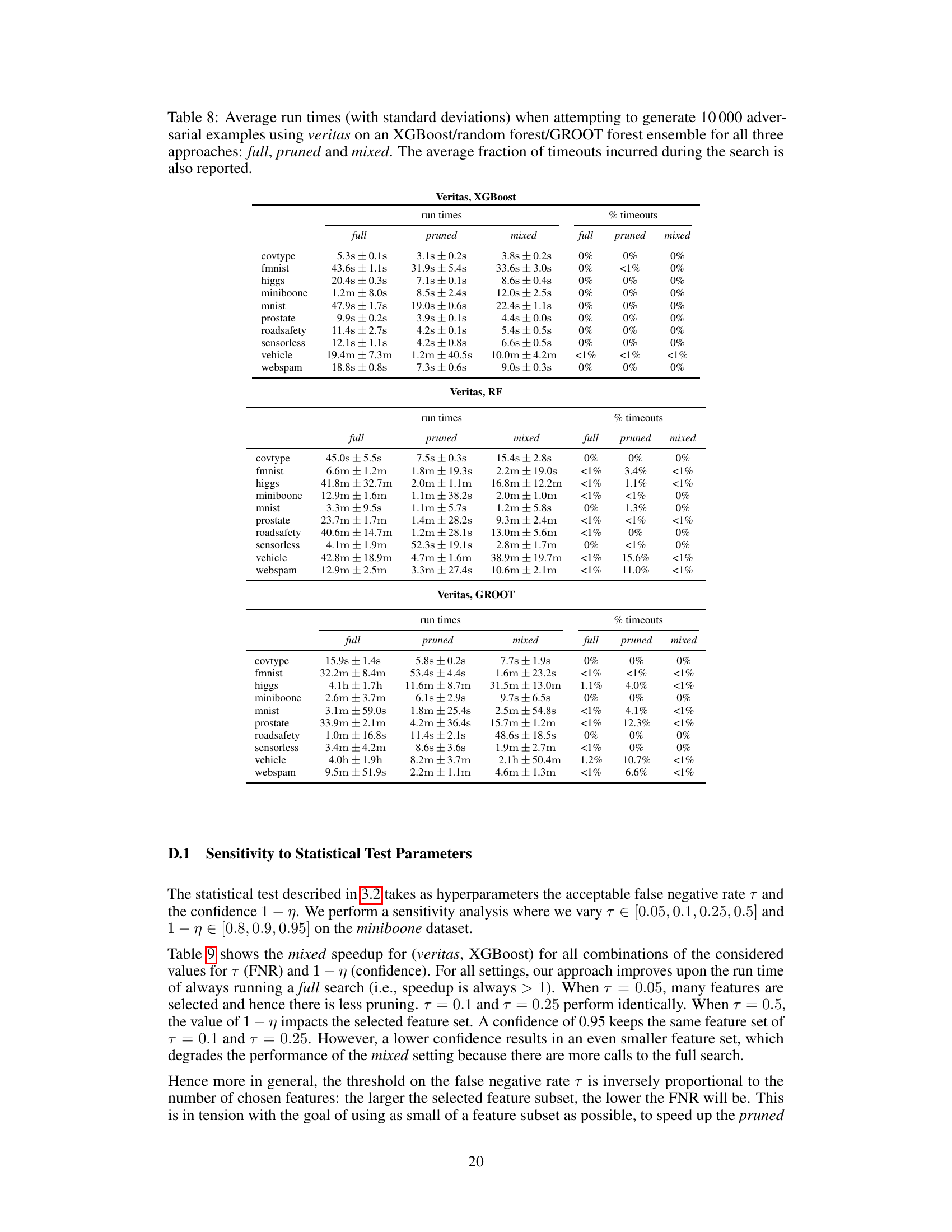
🔼 This table presents the average runtime and speedup achieved by applying three different approaches (full, pruned, and mixed) to generate 10,000 adversarial examples using two different attack methods (kantchelian and veritas) on two different types of tree ensembles (XGBoost and random forest). The speedup is calculated relative to the ‘full’ approach which does not use any optimization techniques. A ‘*’ indicates that the experiment did not complete within the six-hour time limit.
read the caption
Table 2: Average run times and speedups when attempting to generate 10000 adversarial examples using kantchelian/veritas on an XGBoost/random forest ensemble for full, pruned and mixed. A * means that the dataset exceeded the global timeout of six hours.

🔼 This table presents the characteristics of the ten datasets used in the experiments. It shows the number of examples (N), the number of features (#F), the type of classification task (binary or multi-class, converted to binary), the maximum allowed perturbation (δ), and the hyperparameters of the trained models (XGBoost, Random Forest, GROOT). The hyperparameters include maximum tree depth (d), the number of trees (M), learning rate (η for XGBoost), and robustness parameter (ε for GROOT).
read the caption
Table 1: Datasets' characteristics: N and #F are the number of examples and the number of features. higgs and prostate are random subsets of the original, bigger datasets. Multi-class classification datasets were converted to binary classification: for covtype we predict majority-vs-rest, for mnist and fmnist we predict classes 0-4 vs. classes 5-9, and for sensorless classes 0-5 vs. classes 6-10. We also report adopted values of max allowed perturbation δ and learners' tuned hyperparameters after the grid search described in Appendix B. Each ensemble T has maximum tree depth d and contains M trees. The learning rate for XGBoost is η. GROOT robustness is defined by €.

🔼 This table compares the run times of the LT-attack and veritas methods for generating 10000 adversarial examples using a full search. The run times are presented for four datasets: mnist, prostate, roadsafety, and sensorless. The table highlights the significant speed improvement achieved by the veritas method compared to the LT-attack method in the full search setting for adversarial example generation.
read the caption
Table 4: Average run times for generating 10000 adversarial examples using LT-attack and veritas in the full search setting.
🔼 This table presents the average runtime and speedup achieved by using three different approaches (full, pruned, and mixed) for generating 10000 adversarial examples using two different attack methods (kantchelian and veritas) on two different ensemble types (XGBoost and Random Forest). The speedup is calculated by comparing the runtime of the pruned and mixed approaches to the runtime of the full approach. A star (*) indicates that the dataset exceeded the allocated time limit of six hours. The results are presented for several datasets, allowing for a comprehensive analysis of the methods’ performance under different circumstances.
read the caption
Table 2: Average run times and speedups when attempting to generate 10000 adversarial examples using kantchelian/veritas on an XGBoost/random forest ensemble for full, pruned and mixed. A * means that the dataset exceeded the global timeout of six hours.
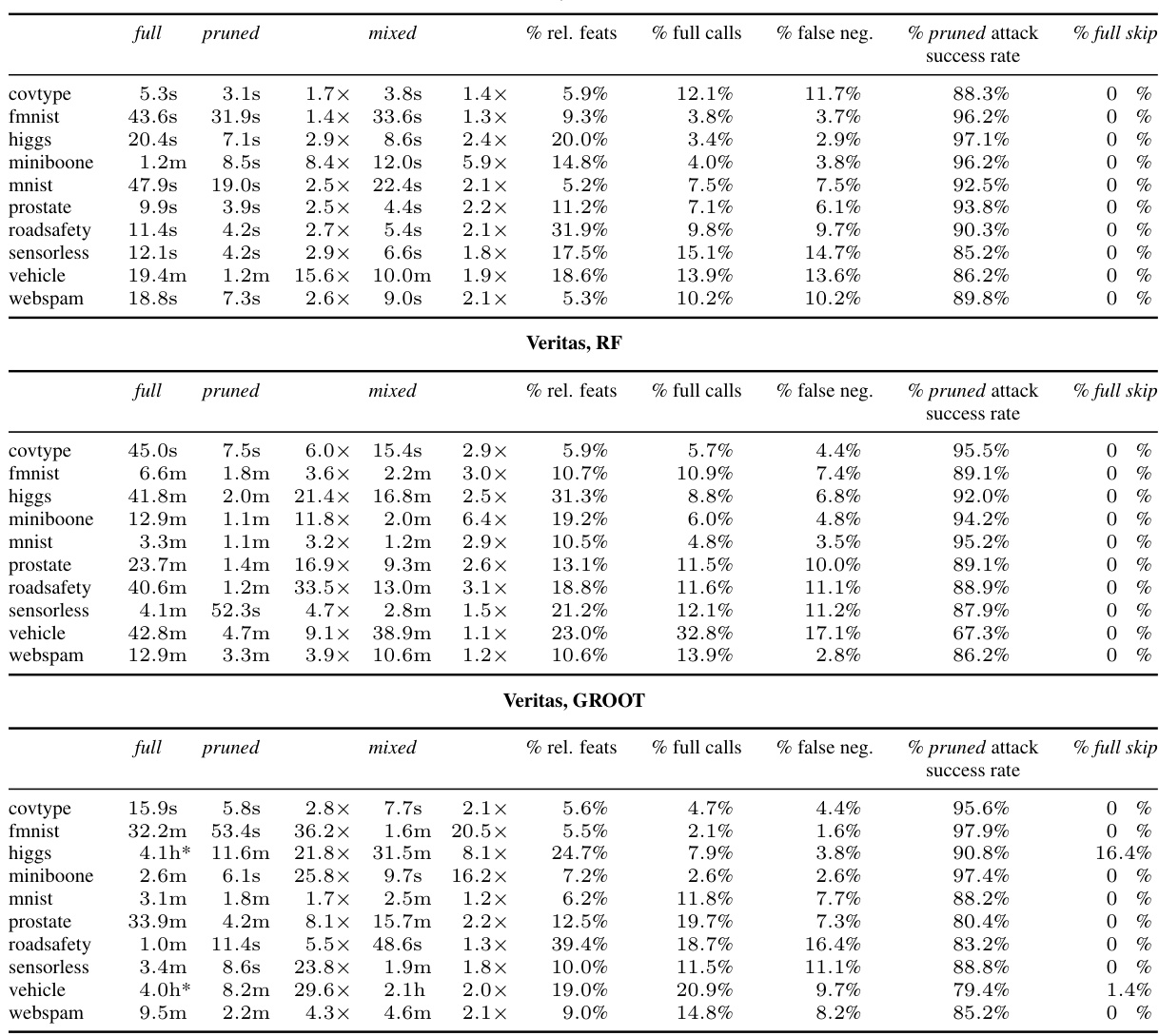
🔼 This table presents the average run time performance of generating 10000 adversarial examples using two different attack methods (kantchelian and veritas) and three different model types (XGBoost, random forest, and a robustified ensemble type GROOT). The table compares the runtime for three different approaches: the original ‘full’ approach, a ‘pruned’ approach that restricts modifications to a subset of frequently perturbed features, and a ‘mixed’ approach that uses the pruned approach first and falls back to the full approach only when necessary. The table shows that the pruned and mixed approaches offer significant speedups over the full approach, especially for Random Forest models. The ‘*’ indicates that the dataset exceeded the time limit of six hours for the full search.
read the caption
Table 2: Average run times and speedups when attempting to generate 10000 adversarial examples using kantchelian/veritas on an XGBoost/random forest ensemble for full, pruned and mixed. A * means that the dataset exceeded the global timeout of six hours.

🔼 This table presents the average runtime and speedup achieved by using three different approaches (full, pruned, and mixed) for generating 10,000 adversarial examples using two different attack methods (kantchelian and veritas) on two different ensemble types (XGBoost and random forest). The speedup is calculated relative to the ‘full’ approach, which doesn’t use any of the optimizations proposed in the paper. The table shows the runtime for each approach on several datasets, highlighting the significant speed improvements achieved by the pruned and mixed methods. An asterisk (*) indicates datasets where the full approach exceeded the six-hour time limit.
read the caption
Table 2: Average run times and speedups when attempting to generate 10000 adversarial examples using kantchelian/veritas on an XGBoost/random forest ensemble for full, pruned and mixed. A * means that the dataset exceeded the global timeout of six hours.

🔼 This table presents the average run times for generating 10000 adversarial examples using two different attack methods (kantchelian and veritas) on two different ensemble types (XGBoost and Random Forest). It compares the performance of three approaches: full (original method), pruned (proposed method), and mixed (combination of full and pruned). The table shows that the proposed methods (pruned and mixed) significantly reduce the runtime compared to the full approach, especially for larger datasets. A ‘*’ indicates that the experiment exceeded the six-hour time limit.
read the caption
Table 2: Average run times and speedups when attempting to generate 10000 adversarial examples using kantchelian/veritas on an XGBoost/random forest ensemble for full, pruned and mixed. A * means that the dataset exceeded the global timeout of six hours.
🔼 This table presents the average runtime and speedup achieved by using three different methods (full, pruned, and mixed) to generate 10,000 adversarial examples using two different attack algorithms (kantchelian and veritas) on XGBoost and random forest ensemble models. The speedup is calculated by comparing the runtime of the pruned and mixed methods to the runtime of the full method. A ‘*’ indicates that the experiment timed out before completion (exceeded a six-hour limit).
read the caption
Table 2: Average run times and speedups when attempting to generate 10000 adversarial examples using kantchelian/veritas on an XGBoost/random forest ensemble for full, pruned and mixed. A * means that the dataset exceeded the global timeout of six hours.

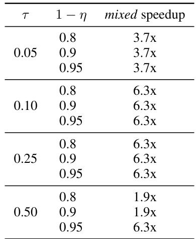
🔼 This table shows the impact of varying the timeout value for the pruned setting (tprun) on the performance of the pruned and mixed approaches. It presents the percentage of timeouts observed in the pruned setting, as well as the speedup factors achieved by the pruned and mixed approaches relative to the full approach for different timeout values. The results demonstrate a trade-off: a smaller timeout leads to fewer timeouts but lower speedups, while a larger timeout results in more timeouts but higher speedups. The optimal timeout value balances speed improvements with the number of timeouts.
read the caption
Table 10: Fraction of pruned timeouts and speedup of the pruned and mixed settings when attempting to generate 10000 adversarial examples for fmnist using (veritas, random forest), for different values of the pruned setting timeout tprun (in seconds).

🔼 This table presents the average run time in seconds for generating 10000 adversarial examples using two different attack methods (kantchelian and veritas) and three different ensemble types (XGBoost, random forest). For each combination of attack method and ensemble type, the table displays the average run time for three different experimental settings: full (original method), pruned (proposed method with feature subset selection), and mixed (combination of the full and pruned methods). The table also indicates cases where the runtime exceeded the 6 hour time limit with a *. Speedup is calculated by comparing the average runtime for the full setting to the average run times for the pruned and mixed settings. This table helps in evaluating the efficiency gains of the proposed feature subset selection method.
read the caption
Table 2: Average run times and speedups when attempting to generate 10000 adversarial examples using kantchelian/veritas on an XGBoost/random forest ensemble for full, pruned and mixed. A * means that the dataset exceeded the global timeout of six hours.

🔼 This table presents the average run time and speedup achieved by using three different approaches (full, pruned, and mixed) to generate 10000 adversarial examples using two different attack methods (kantchelian and veritas) on two different types of ensembles (XGBoost and random forest). The speedup is calculated by comparing the runtime of each approach to the runtime of the full approach. A * indicates that the dataset exceeded the global timeout of 6 hours. The results demonstrate the significant speedup achieved by the pruned and mixed settings across various datasets and ensemble types.
read the caption
Table 2: Average run times and speedups when attempting to generate 10000 adversarial examples using kantchelian/veritas on an XGBoost/random forest ensemble for full, pruned and mixed. A * means that the dataset exceeded the global timeout of six hours.
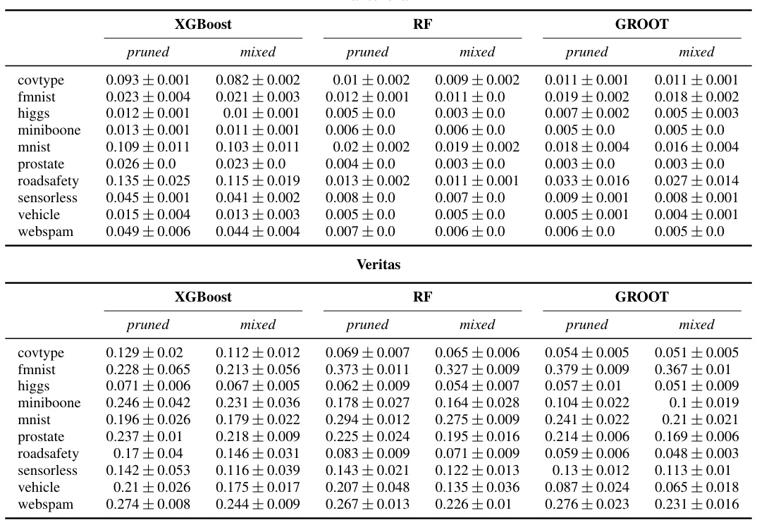
🔼 This table presents the average runtime and speedup achieved by using three different approaches (full, pruned, and mixed) to generate 10000 adversarial examples using two different attack methods (kantchelian and veritas) on two types of ensemble models (XGBoost and random forest). The speedup is calculated relative to the ‘full’ approach. A ‘*’ indicates that the experiment exceeded the six-hour time limit.
read the caption
Table 2: Average run times and speedups when attempting to generate 10000 adversarial examples using kantchelian/veritas on an XGBoost/random forest ensemble for full, pruned and mixed. A * means that the dataset exceeded the global timeout of six hours.
Full paper#


