↗ OpenReview ↗ NeurIPS Homepage ↗ Chat
TL;DR#
Many machine learning models struggle with distribution shifts, where training and deployment data differ significantly. Distributionally Robust Optimization (DRO) tackles this by finding solutions that perform well across various data distributions. However, existing DRO algorithms often lack efficiency and struggle with large datasets and complex uncertainty sets. These limitations hinder their practical use in real-world scenarios, which often involve high-dimensional datasets and unpredictable data distributions.
This paper introduces DRAGO, a novel stochastic primal-dual algorithm, designed to overcome these challenges. DRAGO utilizes variance reduction and incorporates both cyclic and randomized updates to achieve linear convergence. This significant improvement in speed and efficiency is demonstrated both theoretically and empirically, outperforming existing approaches. DRAGO shows strong performance across various uncertainty sets and real-world datasets, making it a highly practical tool for real-world DRO applications. The superior complexity guarantee is supported by a detailed theoretical analysis and extensive experiments.
Key Takeaways#
Why does it matter?#
This paper is crucial for researchers working on distributionally robust optimization (DRO), a vital area in machine learning dealing with data uncertainty. It offers a novel algorithm, DRAGO, achieving state-of-the-art linear convergence with fine-grained dependency on problem parameters, surpassing existing methods. It also expands to broader applications beyond DRO, impacting related fields like min-max optimization. The provided theoretical analysis, open-source code, and comprehensive experiments enhance reproducibility and encourage further research in DRO and its applications.
Visual Insights#

This figure visualizes how the uncertainty set and penalty term in the penalized DRO objective function interact to define an effective uncertainty set. Each plot shows a probability simplex (a triangle in 3 dimensions) where the colored area represents the uncertainty set Q. The black dots are optimal dual variables q* which maximize the objective for a given primal variable w. As the penalty parameter v decreases, the optimal dual variable q* can move closer to the boundary of the uncertainty set. The choice of divergence function D and penalty parameter v together determine the shape of this effective uncertainty set.
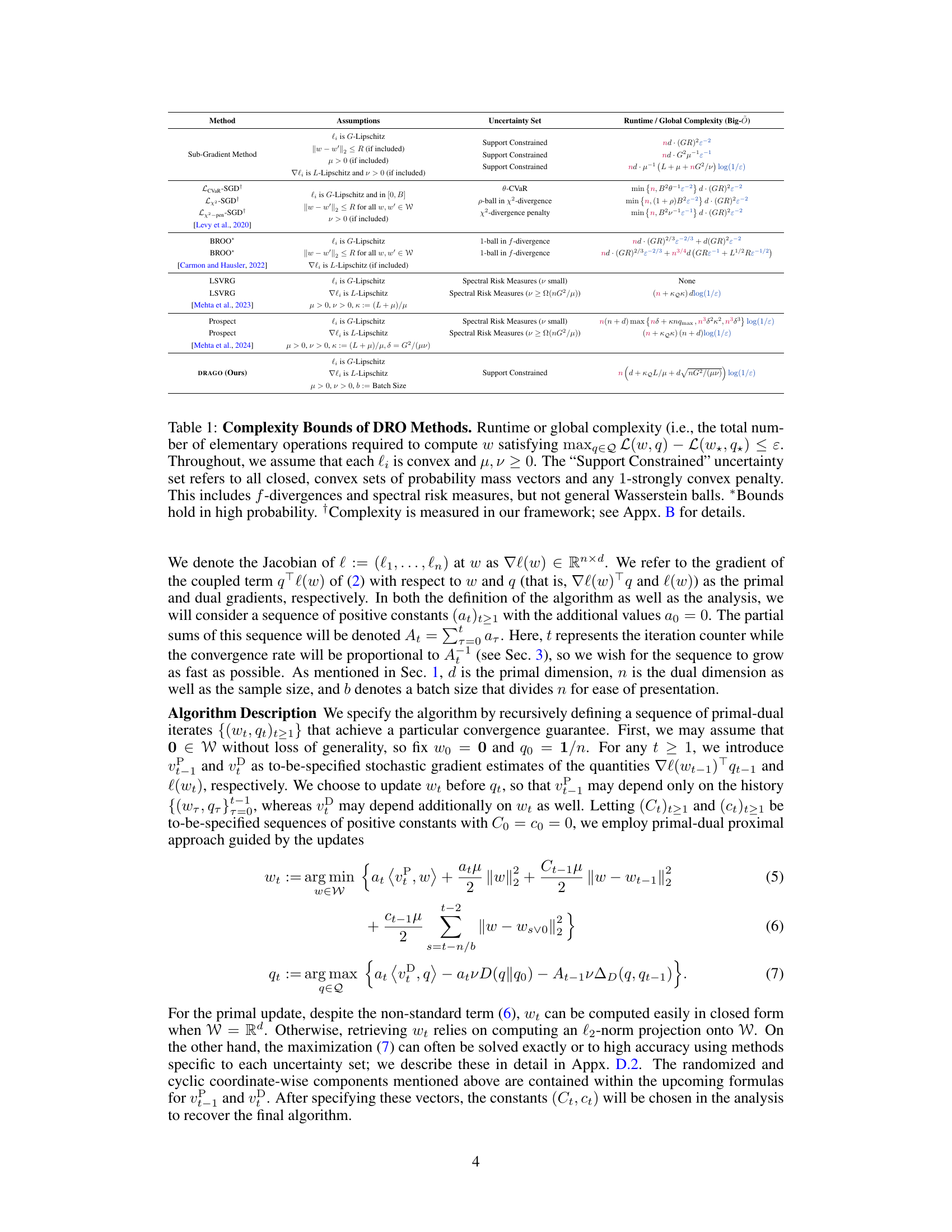
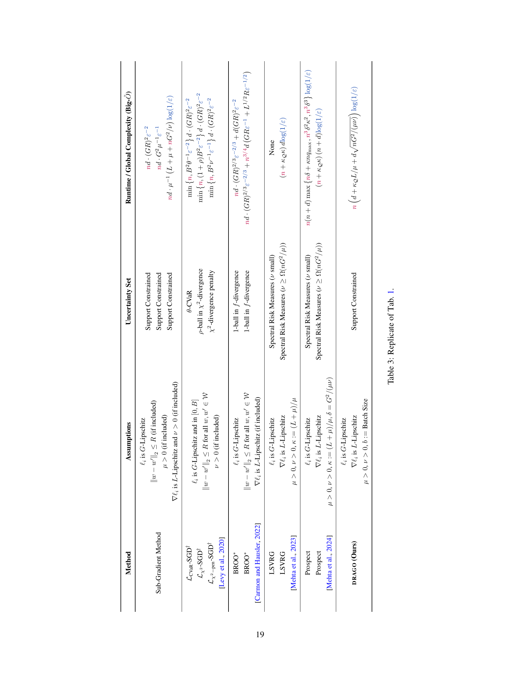
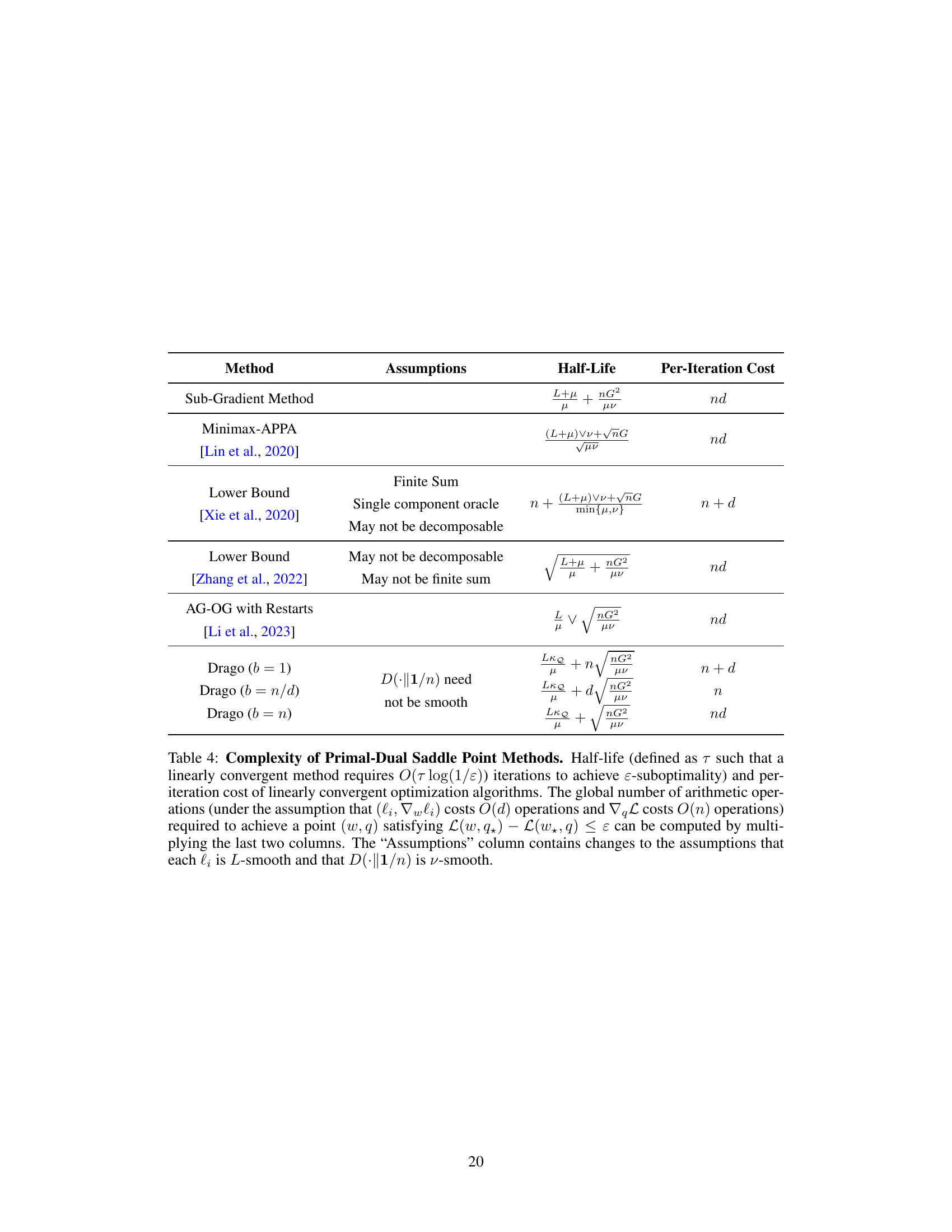
This table compares the computational complexity of various DRO methods in terms of the total number of operations needed to reach an ϵ-optimal solution for the penalized DRO problem. It presents different methods, their assumptions, the type of uncertainty sets they handle, and their corresponding complexities. The complexities are expressed using Big-O notation and show the dependence on parameters like sample size (n), dimension (d), Lipschitz constants (G, L), and regularization parameters (μ, ν). It also highlights the differences in complexities when different uncertainty sets (e.g., support-constrained, f-divergence based, spectral risk measures) are considered.
In-depth insights#
DRAGO Algorithm#
The DRAGO algorithm, a stochastic primal-dual approach for distributionally robust optimization (DRO), presents a novel solution for handling the complexities of DRO problems. Its key innovation lies in combining cyclic and randomized components with a carefully regularized primal update, which leads to dual variance reduction. This design is crucial for achieving linear convergence, a significant improvement over existing sublinear methods. By using minibatch stochastic gradient estimates, DRAGO efficiently balances per-iteration computational cost with the number of iterations required to reach a solution. The algorithm’s flexibility extends to handling a wide range of uncertainty sets, showcasing its adaptability and practicality for real-world applications. The theoretical analysis supporting DRAGO demonstrates a fine-grained dependency on condition numbers, providing a strong theoretical foundation. Importantly, its performance is demonstrably superior to existing methods, particularly in the high-dimensional settings and ill-conditioned problems often encountered in DRO applications, making it a powerful and efficient tool for solving large-scale distributionally robust optimization problems.
DRO Complexity#
Analyzing the complexity of Distributionally Robust Optimization (DRO) problems reveals crucial insights into their computational feasibility. The sample size (n) significantly impacts runtime, often dominating the complexity in many algorithms. The dimensionality (d) of the problem also plays a role, although its influence is often less pronounced than n. Existing DRO algorithms exhibit varying complexities; some achieve sublinear rates (e.g., O(ε⁻²)), while others, especially variance-reduced methods, can achieve linear convergence under specific assumptions like strong convexity. The choice of uncertainty set and divergence measure significantly affects the algorithm’s complexity, with some settings being considerably harder than others. For instance, Wasserstein DRO often presents more computational challenges than f-divergence based DRO. The strong convexity and smoothness of the objective function significantly influence the convergence rate, with strongly convex and strongly concave problems generally enjoying faster convergence. The development of efficient algorithms with fine-grained complexity analysis that accounts for these factors remains a significant challenge in the field, necessitating further research.
Empirical Results#
An Empirical Results section in a research paper should present a thorough evaluation of the proposed method, comparing its performance against relevant baselines across various metrics. Strong emphasis should be placed on clear visualization, using graphs and tables that effectively showcase the findings. The datasets used should be carefully described, highlighting their characteristics and size. A discussion of hyperparameter tuning is crucial, explaining the methodology employed and its influence on the results. Statistical significance testing should be incorporated to confirm the reliability and robustness of observed improvements. Furthermore, a detailed analysis of computational efficiency is necessary, including runtimes and memory usage, offering insights into practical applicability. Finally, concise conclusions that summarize the key observations and their implications for the research field are vital. The section should be comprehensive, presenting both positive and negative aspects of the empirical results to maintain objectivity.
Future Research#
The paper’s main contribution is a novel algorithm called DRAGO for faster distributionally robust optimization. Future research could explore extensions to non-convex settings, which are often encountered in real-world applications. Another promising avenue is applying DRAGO to min-max problems beyond distributional robustness, such as missing data imputation and fully composite optimization. The algorithm’s dependence on specific types of uncertainty sets suggests a need for investigation of more general uncertainty set handling. Additionally, a thorough empirical evaluation across a wider range of datasets and hyperparameter settings would further strengthen the claims made. Finally, research could delve into the theoretical properties more deeply, such as tighter complexity bounds and the analysis of convergence rates under weaker assumptions.
Method Limits#
A hypothetical ‘Method Limits’ section in a research paper would critically examine the boundaries and shortcomings of the proposed methodology. It would delve into aspects like computational complexity, acknowledging potential limitations in scaling to very large datasets or high-dimensional feature spaces. The discussion would also address the assumptions underpinning the method, such as strong convexity or smoothness of the objective function, highlighting scenarios where these assumptions might not hold and the method’s performance could degrade. Furthermore, a thoughtful analysis would assess the generalizability of the method across various problem domains or data distributions, and explore situations where the method might be less effective. Finally, a discussion of potential biases introduced by the method or limitations in its interpretability would also be vital. Essentially, this section would provide a nuanced perspective, balancing the method’s strengths with a clear-eyed view of its limitations.
More visual insights#
More on figures

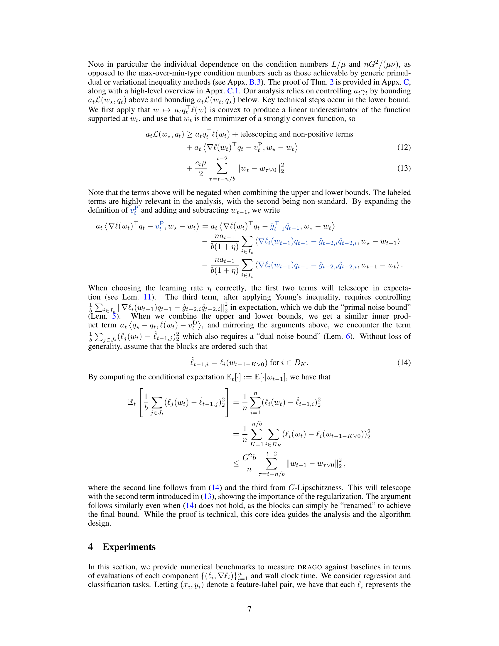
This figure presents the results of regression experiments on six different datasets using three different optimization algorithms: SGD, LSVRG, and DRAGO. The left panel shows the primal suboptimality gap (a measure of how close the algorithm is to the optimal solution) plotted against the number of first-order oracle calls (a measure of computational cost). The right panel shows the same primal suboptimality gap plotted against the wall-clock time (a measure of real-world time). The different lines represent the different algorithms. This figure shows the performance of the algorithms in terms of both computational cost and real-world time.

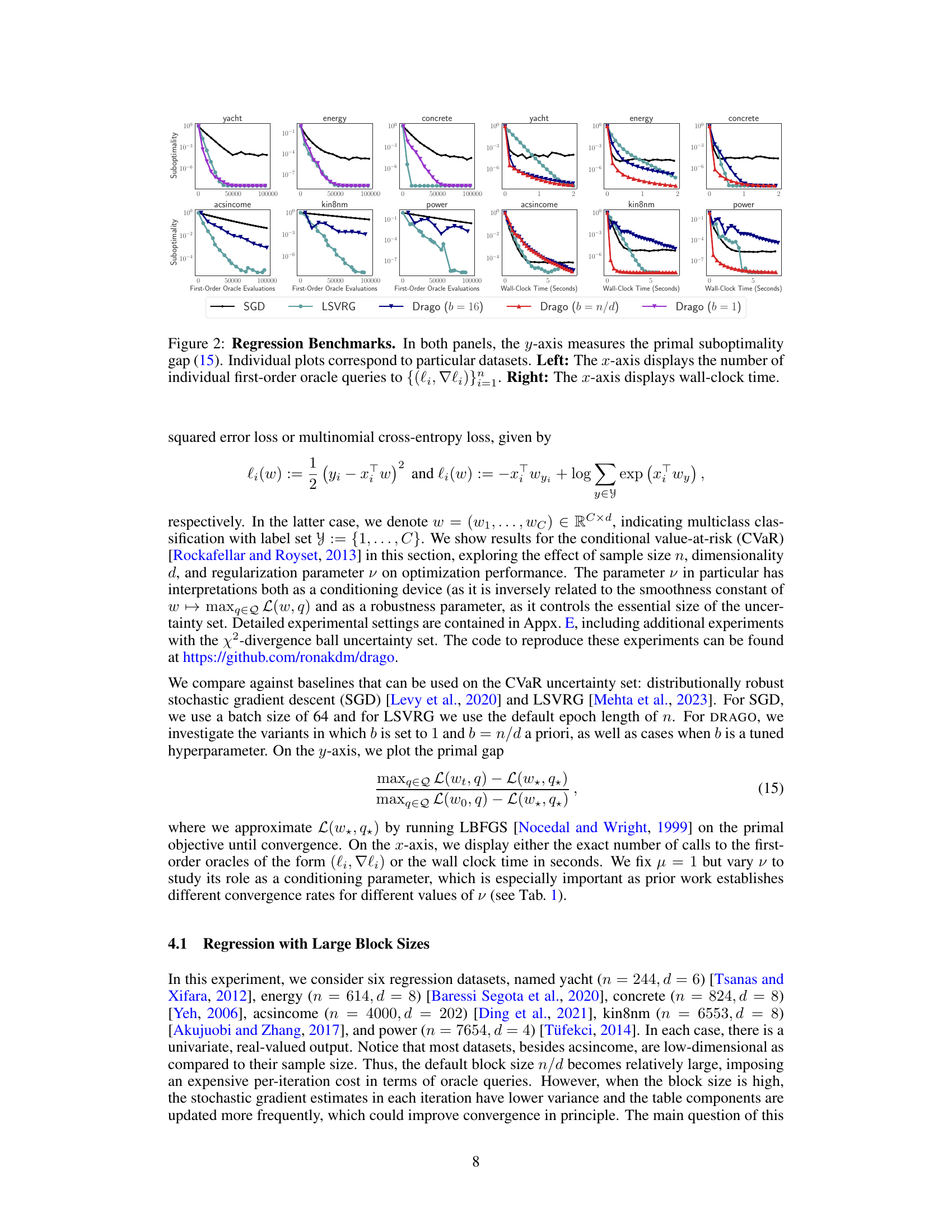
The figure presents the results of text classification experiments using DRAGO, comparing its performance against baselines for different values of the dual regularization parameter (v). The plots show the normalized primal suboptimality gap (a measure of convergence) against the number of first-order oracle queries and wall-clock time. The results are shown for various values of v, demonstrating DRAGO’s performance under different levels of ill-conditioning. The left panels show the suboptimality against the number of gradient calls, while the right panels show it against the wall-clock time.

This figure presents the results of regression experiments comparing DRAGO with different batch sizes (b=1, 16, n/d) against standard SGD and LSVRG methods. The left panel shows the primal suboptimality gap (a measure of optimization progress) plotted against the number of first-order oracle calls (a measure of computational cost). The right panel shows the same suboptimality gap but against wall-clock time, offering a more practical comparison that includes the overhead associated with the various algorithms. Each sub-plot corresponds to a different regression dataset, allowing for a comparison across various data characteristics.
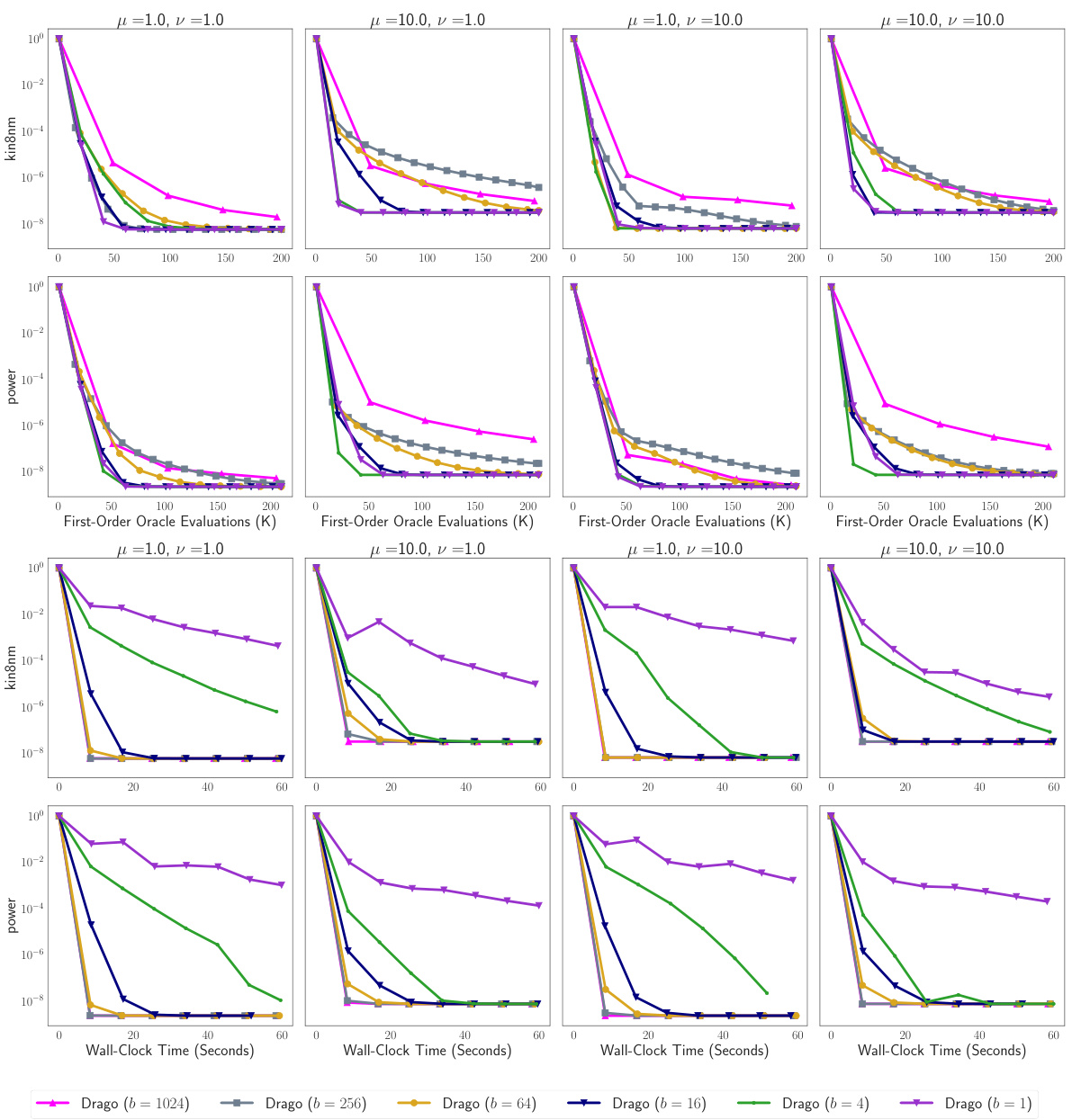
The figure shows the impact of batch size and strong convexity parameters on DRAGO’s performance across different datasets. The top rows show the number of first-order oracle queries (a measure of computational cost), while the bottom rows display the wall-clock time. Each row represents a specific dataset, and each column shows the results for a different combination of strong convexity regularization parameters (μ and ν). The results illustrate the trade-off between computational cost and wall-clock time for varying batch sizes.
More on tables
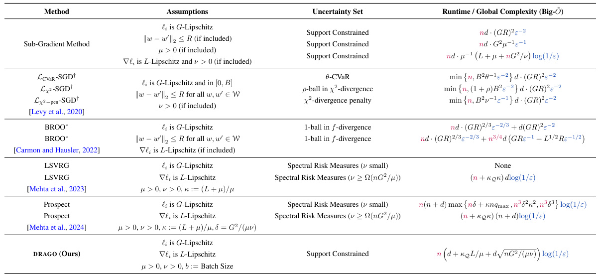
This table compares the complexity of various DRO methods in terms of runtime or global complexity. It shows the assumptions made by each method, the type of uncertainty set used, and the resulting complexity bound. The complexity is expressed in Big-Õ notation and accounts for the number of elementary operations needed to reach an Ɛ-optimal solution. The table highlights the dependence of each method’s complexity on the sample size (n), dimension (d), and relevant constants, such as smoothness and strong convexity parameters.
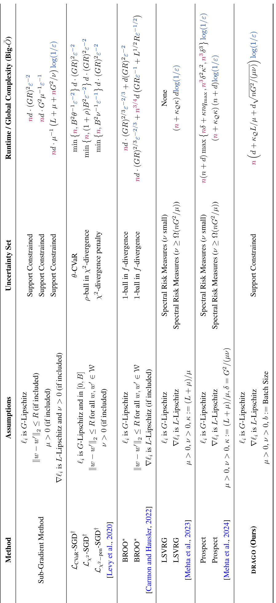
This table compares the complexity of various DRO methods. It shows the runtime or global complexity (total number of operations) needed to achieve an ϵ-optimal solution for different methods under various assumptions and uncertainty set types. Key factors influencing complexity, such as sample size (n), dimension (d), Lipschitz constants (G, L), strong convexity parameters (μ, ν), and batch size (b), are included. Note that the complexity measures are given in Big-Õ notation and that some bounds are high-probability guarantees. The table also specifies the type of uncertainty set considered (e.g., support constrained, f-divergence, spectral risk measures).
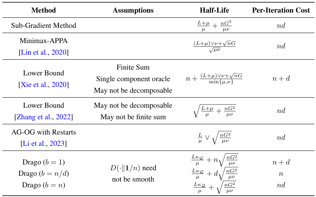
This table compares the complexity of various DRO methods in terms of runtime or global complexity. It shows the assumptions made by each method, the type of uncertainty set it handles, and its resulting complexity bound. The complexity is expressed using Big-Õ notation and depends on factors like sample size (n), dimensionality (d), Lipschitz constants (G,L), regularization parameters (μ,ν), and the size of the uncertainty set (kQ). The table highlights the trade-offs between different methods and their suitability for various problem settings. Note that some bounds hold with high probability.
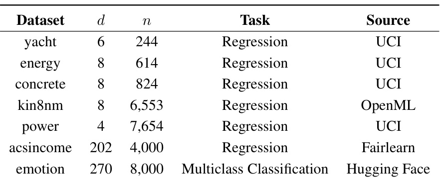
This table compares the computational complexity of various DRO methods in terms of the total number of elementary operations needed to achieve an ϵ-optimal solution. It lists different methods, their assumptions (e.g., Lipschitz continuity of loss functions, strong convexity), the type of uncertainty set they handle, and their runtime/global complexity. The complexity is expressed using Big-Õ notation and highlights the dependence on sample size (n), dimension (d), and other relevant parameters like smoothness constants and the size of the uncertainty set.
Full paper#
