↗ OpenReview ↗ NeurIPS Homepage ↗ Chat
TL;DR#
Many AI tasks struggle with causal reasoning due to a mismatch between data granularity and high-level causal variables. Existing causal methods often assume data as granular as underlying causal factors. This paper tackles the problem of causal disentangled representation learning in non-Markovian settings with multiple domains. It highlights the need for methods that can handle such complexities.
The paper introduces graphical criteria to determine variable disentanglement under various conditions. It proposes CRID, an algorithm that leverages these criteria to produce a causal disentanglement map, showing which latent variables are disentangled given available data and assumptions. Empirical results on simulations and MNIST datasets validate CRID’s performance and demonstrate its ability to achieve disentanglement in non-trivial settings.
Key Takeaways#
Why does it matter?#
This paper is crucial for AI researchers working on causal representation learning and disentanglement. It addresses a critical gap in existing methods by handling non-Markovian systems and heterogeneous data, offering both theoretical insights and practical algorithms. This opens new avenues for building more robust and generalizable AI systems capable of performing sophisticated reasoning tasks.
Visual Insights#
This figure illustrates the process of learning disentangled causal latent representations from heterogeneous data and assumptions. It shows a data generating model where high-dimensional data (e.g., images, text) X is a non-linear transformation of lower-dimensional latent variables V, which represent causal factors. The latent causal graph (LCG) depicts the causal relationships between these latent variables V. The goal is to learn the inverse of the mixing function (f⁻¹) to obtain disentangled representations of the latent causal variables, highlighting which latent variables can be separated from others given the data and causal assumptions. This disentanglement is crucial for various downstream AI tasks.

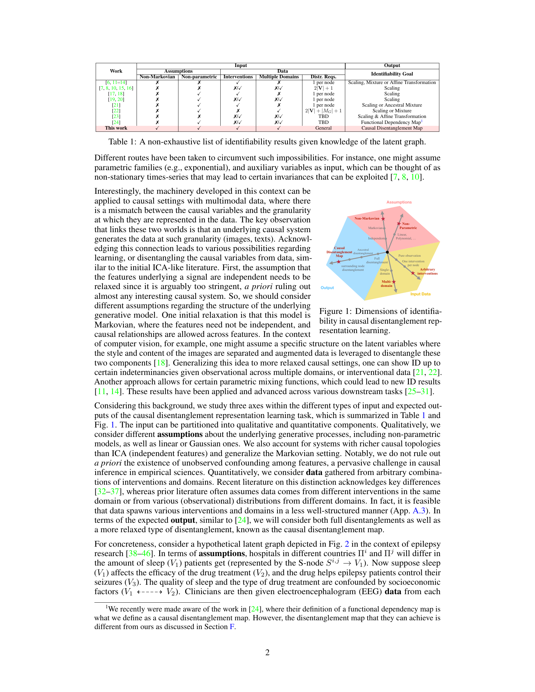
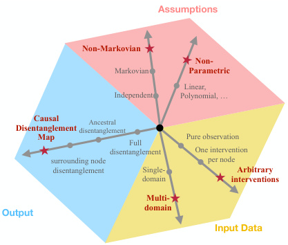
This table compares various works in causal disentangled representation learning, highlighting their assumptions, input data types (observational and interventional), handling of multiple domains, and the identifiability goals achieved. It shows whether each work considers non-Markovian settings, utilizes non-parametric methods, requires specific input interventions, and addresses multiple data domains. The ‘Distr. Reqs’ column indicates the number of distributions required for identifiability results. Finally, the ‘Identifiability Goal’ column indicates the level of disentanglement achieved, ranging from full disentanglement to functional dependency maps.
In-depth insights#
Causal Disentanglement#
Causal disentanglement, a critical concept in causal representation learning, seeks to decompose complex data into its underlying causal factors, enabling a better understanding of cause-and-effect relationships. This is particularly challenging when dealing with high-dimensional data like images or text, where observed variables are often at a different granularity than the underlying causal variables. The key goal is to learn representations where these latent causal variables are disentangled, allowing for improved prediction, fairness, and generalizability. Non-Markovian settings, involving unobserved confounding, pose a significant challenge, demanding new graphical criteria and algorithms to determine disentanglement. The combination of data from multiple heterogeneous domains further complicates the task, making it necessary to account for domain-specific variations. Successful causal disentanglement hinges on carefully considering these challenges and developing methods that handle both the richness of the causal structure and the diverse nature of the input data.
Non-Markovian Setting#
The concept of a ‘Non-Markovian Setting’ in the context of causal inference signifies a departure from the Markovian assumption, which posits that the future is conditionally independent of the past given the present. In Non-Markovian systems, the past directly influences the future, even when the present state is known. This introduces complexities into causal reasoning because standard methods designed for Markovian processes may not provide accurate or reliable results. Unobserved confounding plays a significant role in Non-Markovian settings, making it difficult to isolate true causal effects. The presence of latent variables, which are unobserved, further complicates analysis. Therefore, analyzing and learning causal relationships within a Non-Markovian setting necessitate techniques that explicitly consider the temporal dependencies and potential influences of the past on the future, and address the challenges posed by unobserved variables and confounding.
Multi-Domain Analysis#
Multi-domain analysis in research papers often involves investigating phenomena across diverse datasets or settings. This approach is crucial when a single dataset isn’t representative enough to capture the full scope of a problem. A key strength is the potential for increased generalizability of findings. By analyzing data from different domains, researchers can identify patterns and relationships that hold true across various contexts, making their conclusions more robust and less susceptible to biases from limited sampling. However, challenges exist. Data harmonization is vital; ensuring consistency and comparability across diverse data sources requires careful planning and methodology, often including standardized data formats and transformations. Furthermore, statistical analysis needs to account for potential domain-specific effects; naively pooling data might mask important differences or lead to spurious results. Careful consideration of confounding factors is also critical, as these could vary between domains, confounding the causal relationships of interest. Careful interpretation is necessary to avoid overgeneralizing findings from one domain to another. Despite these challenges, the insights gained from multi-domain analysis can be immensely valuable in achieving a more comprehensive and nuanced understanding of a topic.
CRID Algorithm#
The CRID algorithm, designed for causal disentanglement mapping, systematically determines the disentangleability of latent variables. It leverages a latent selection diagram and interventional data to identify which latent variables can be disentangled. CRID’s strength lies in its ability to handle non-Markovian settings and heterogeneous data, which are common in real-world AI applications. The algorithm incorporates graphical criteria to assess disentanglement under various conditions, and its theoretical foundation is supported by experimental results. The algorithm’s novelty stems from its ability to handle multiple domains and non-Markovian causal settings, going beyond limitations of prior approaches. The results corroborate the theory, demonstrating CRID’s practical applicability. However, its reliance on the accuracy of the latent causal graph remains a crucial limitation. Future work could explore ways to integrate latent structure learning within the CRID framework.
Future Directions#
Future research could explore several promising avenues. Extending the framework to handle unknown causal structures is crucial, moving beyond the assumption of a known latent causal graph. This would involve developing methods for simultaneously learning the causal structure and disentangled representations. Another key area is improving the efficiency and scalability of the proposed algorithm, CRID, particularly for high-dimensional data. Investigating the impact of different intervention types and assumptions on disentanglement is important. The current approach assumes certain properties of the mixing function and interventions which can be further relaxed. Addressing the challenges posed by nonlinear and non-Markovian causal systems is needed to broaden the applicability of the framework. Finally, applying the disentangled representations to real-world AI applications, such as image generation, causal inference, and decision making, would demonstrate the practical value of this work. Investigating the tradeoffs between different disentanglement levels and downstream task performance will guide the development of more effective AI systems.
More visual insights#
More on figures
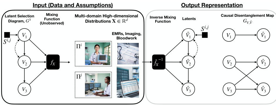
This figure illustrates the process of learning disentangled causal latent representations from heterogeneous data and assumptions. The left side shows the data generating model, which includes latent variables (V1, V2, V3), a mixing function (fx), and observed data (X) from multiple domains. The right side shows the goal of the learning process, which is to obtain a disentangled representation of the latent variables and a causal disentanglement map that highlights the relationships between the latent variables. The figure also shows an example of how the different data modalities (EMRs, imaging, bloodwork) can be used to learn the disentangled representations.
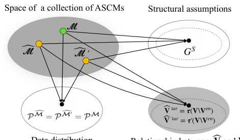
This figure illustrates the process of learning disentangled causal latent representations from heterogeneous data. The data generating model consists of latent variables (V) that are mixed (via a function fx) to produce observed high-dimensional data (X). The goal is to learn the inverse mixing function (fx⁻¹) and a disentangled representation of the latent variables, where some chosen latent variables are disentangled from others. This process is illustrated using a diagram that shows the relationship between the inputs (data and assumptions), the latent selection stage, the mixing process, the inverse mixing, and the causal disentanglement map that is the ultimate output.

This figure illustrates the general framework of causal disentangled representation learning. The left side shows the data generating model, which involves latent variables (V) that are mixed through a nonlinear function (fx) to produce the observed data (X). The right side shows the goal of learning a disentangled causal latent representation, where the latent variables are separated and their relationships are clearly represented. This process involves finding the inverse of the mixing function (f⁻¹) to extract the latent variables from the observed data.

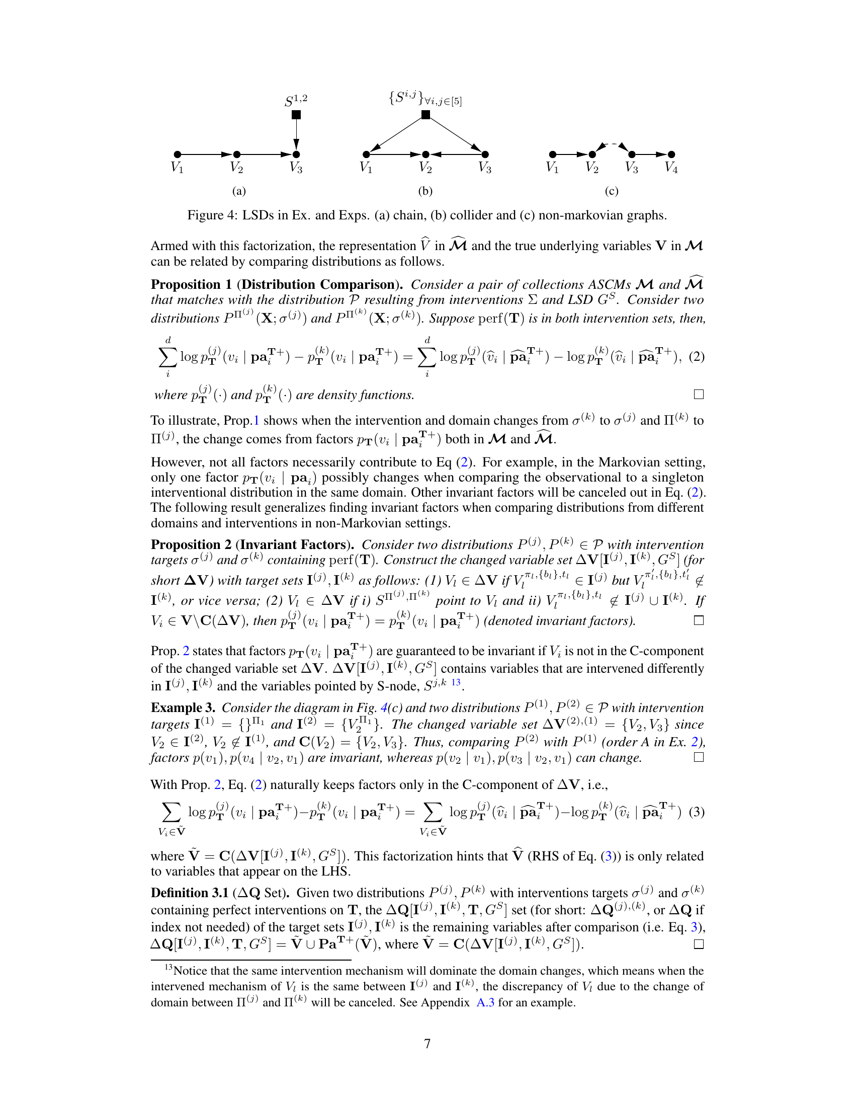
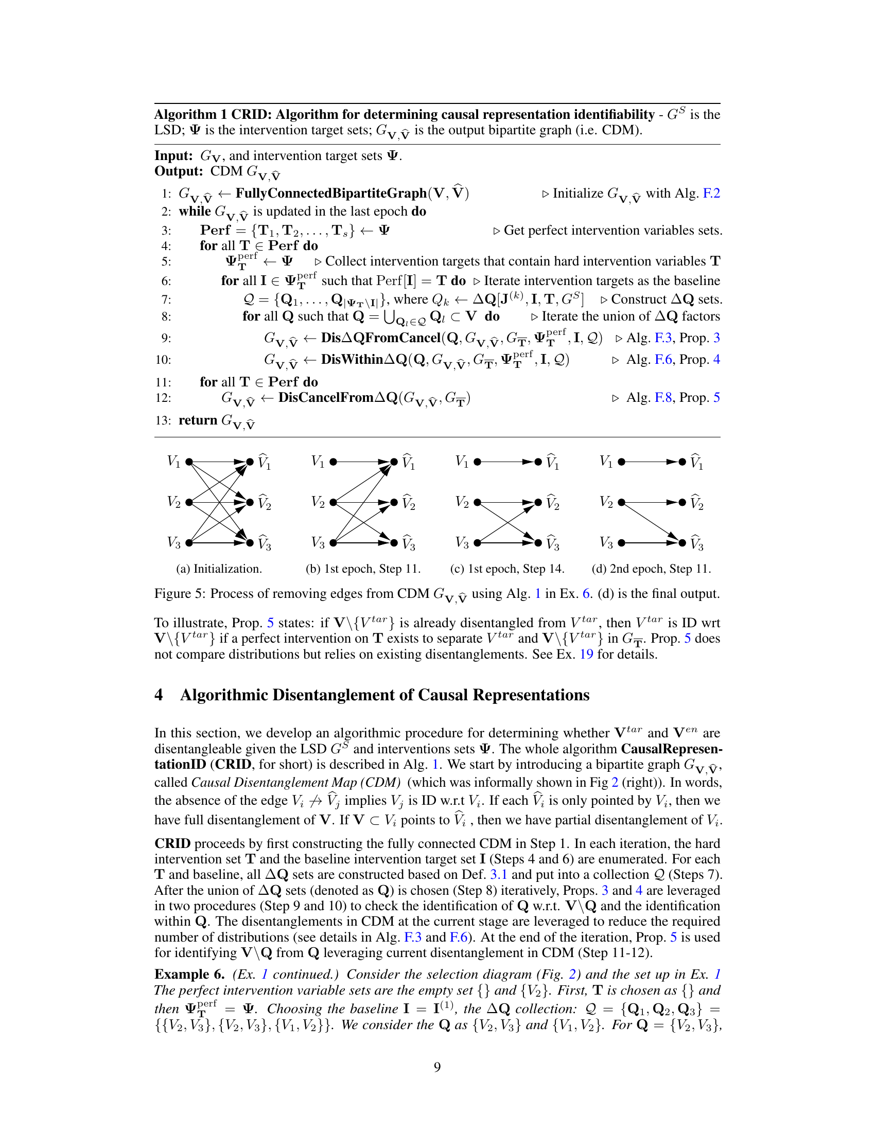
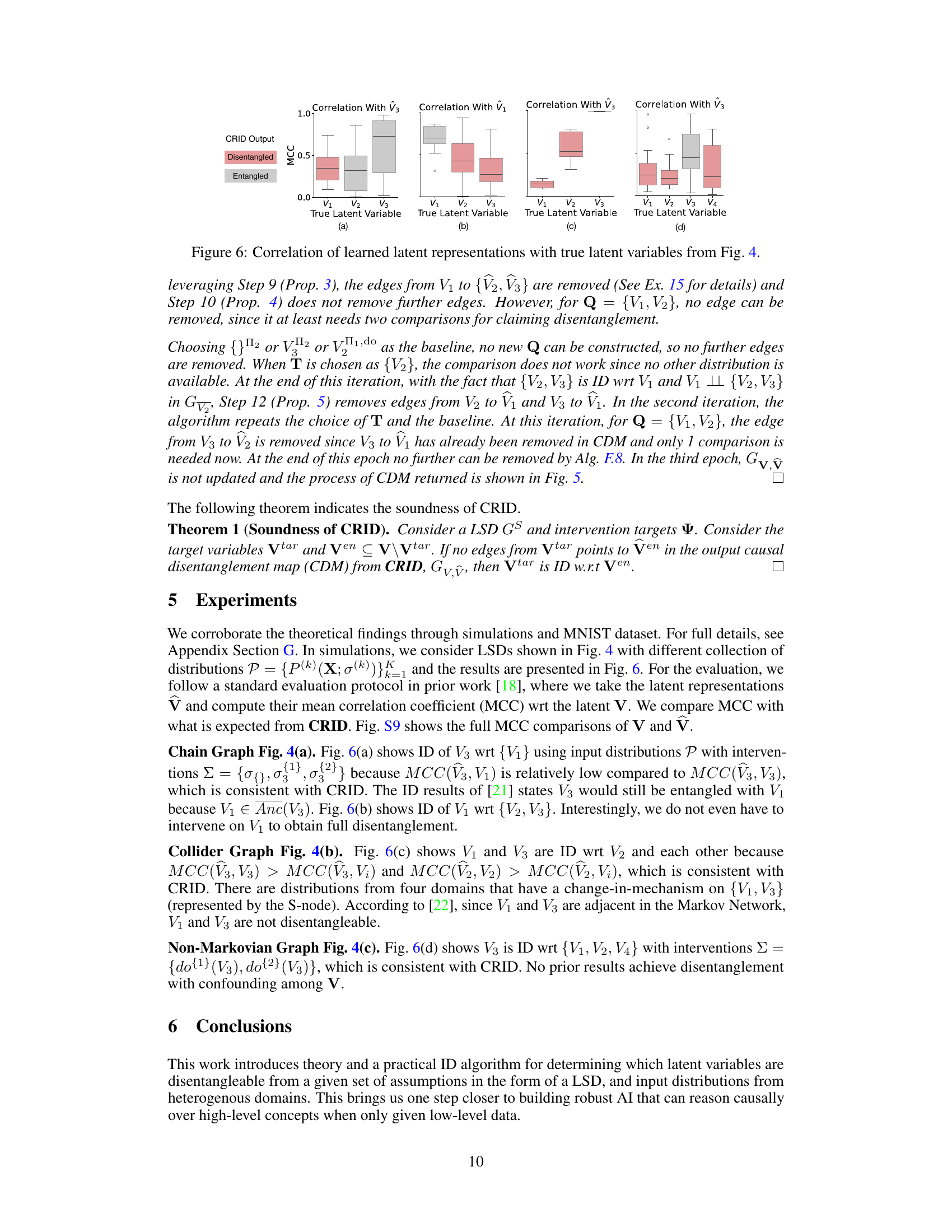
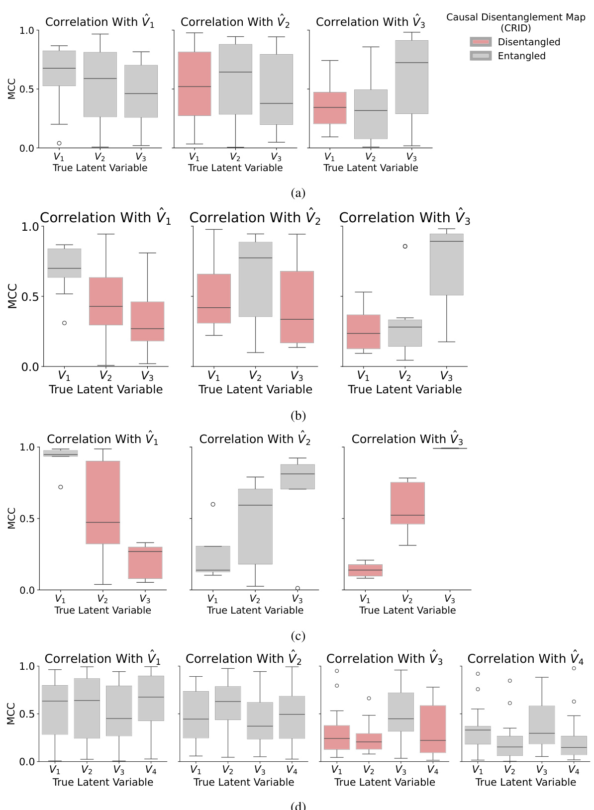
This figure displays the results of experiments on four different causal graphs (chain, collider, non-Markovian, and another non-Markovian graph). Each subplot shows the correlation between the learned latent variables and the ground truth latent variables for a specific causal graph. The mean correlation coefficient (MCC) is used as a metric and visualized using box plots for each latent variable (V1, V2, V3, V4). Red indicates variables predicted by the CRID algorithm to be disentangled from other variables, and gray indicates those predicted to be entangled. The results demonstrate the ability of the CRID algorithm to identify disentangled variables in various causal settings, even in complex non-Markovian scenarios.

The figure illustrates the data generation process and the goal of disentangled representation learning. On the left, a data generating model is shown, which includes a latent causal graph (LCG) representing the relationships between latent variables (V1, V2, V3). These latent variables are mixed through a non-linear function fx to generate high-dimensional data X (e.g., images, text). On the right, the goal of disentangled representation learning is depicted, where the disentangled latent representations are learned from data and assumptions about the underlying causal structure. The disentanglement map Gvv highlights which latent variables can be disentangled given the combination of data and assumptions. The overall goal is to learn the inverse of the mixing function fx and the disentangled latent representations V, where the latent variables (V1, V2, V3) are disentangled given the input distributions and assumptions regarding the causal structure.

This figure illustrates the process of learning disentangled causal latent representations from heterogeneous data and assumptions about the underlying causal system. The left side shows a data generating model with observed data (images, EMRs, bloodwork) arising from a combination of heterogeneous domains. Latent variables (V1, V2, V3) generate the observed data through a nonparametric mixing function (fx). The right side shows the goal of the disentanglement process—to learn the inverse mixing function (f-1) and disentangled latent representations, highlighting which variables can be disentangled given the data and assumptions. This disentanglement is depicted using a causal disentanglement map (Gvv). The figure highlights the challenge of learning realistic causal representations from data with various modalities and the importance of disentangling latent causal variables to ensure accuracy and reliability.

This figure illustrates the process of learning disentangled causal latent representations from heterogeneous data and assumptions. The left side depicts the data generating process, starting with latent causal variables (V1, V2, V3) mixed by a non-linear function fx to produce high-dimensional observed data X, such as images or text. The causal relationships between the latent variables are shown as a directed acyclic graph (DAG). The right side displays the goal of learning disentangled latent representations. The learned representation should ideally mirror the structure of the original causal DAG, separating the latent variables that are causally independent, even if they are correlated in the observed data X. The image shows the input, the process of latent selection and the mixing function, and the final disentangled representation.

This figure illustrates the model for generating data (left panel) and the goal of disentangled causal representation learning (right panel). The data is generated from latent causal variables (V) through a nonlinear mixing function (fx). The goal is to learn the inverse mixing function (f⁻¹) and a disentangled representation of the latent variables, highlighting which latent variables are disentangled from others given the observed data and causal assumptions. The figure shows an example with three latent variables (V₁, V₂, V₃) and their relationships, emphasizing the challenge of learning meaningful representations from high-dimensional data (X) that accurately captures these latent causal relationships.

This figure illustrates the general framework of the proposed causal disentangled representation learning approach. It shows a data generating model where observed high-dimensional data (e.g., images, text) X is generated from latent causal variables V through a nonlinear mixing function fx. The goal of the learning task is to learn the inverse of this function and recover disentangled causal representations of the latent variables, highlighting which latent variables can be disentangled given the combination of data and assumptions encoded in a latent causal graph. The figure depicts the input, which includes data and assumptions in the form of a latent causal graph, and the output, which is a causal disentanglement map that shows the relationships between latent variables.

This figure illustrates the process of learning disentangled causal latent representations. The left side shows a data generating model, where observed data X (e.g., EEG data, images, texts) is a nonlinear transformation of latent causal variables V (e.g., drug, sleep, seizures). The model highlights the presence of a latent causal graph Gvv that describes relationships between these latent variables. The right side represents the goal, which is to learn a causal disentanglement map. This map indicates the relationships between the original variables (V) and the disentangled representation (V), highlighting which variables can be disentangled from others given available data and assumptions regarding the causal structure.
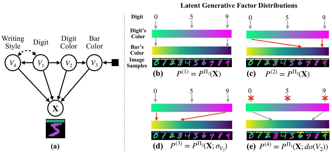
This figure illustrates the data generation process and the goal of learning disentangled causal latent representations. The left side shows a data generating model with latent variables (V1, V2, V3) and an observed mixture variable X. These latent variables are connected in a latent causal graph (LCG). The observed variable X is a nonlinear transformation of the latent variables. The right side depicts the desired output: a causal disentanglement map (CDM) showing which latent variables can be disentangled from each other given the observed data and assumptions. This demonstrates the goal of learning a representation where the latent causal factors are disentangled from each other, facilitating various downstream tasks.
This figure illustrates the process of learning disentangled causal latent representations from heterogeneous data and assumptions. The left side shows a data generating model with latent variables (V1, V2, V3) and observed high-dimensional data (X, e.g., images or text) which are non-linearly mixed by a function fx. The right side shows the desired disentangled representation with a causal disentanglement map (Gvv) which maps the latent variables to their disentangled representations. The Sij nodes represent potential discrepancies in the generative process between different domains or interventions. The overall goal is to learn the inverse function f-1x and obtain a disentangled representation of the latent variables.
More on tables
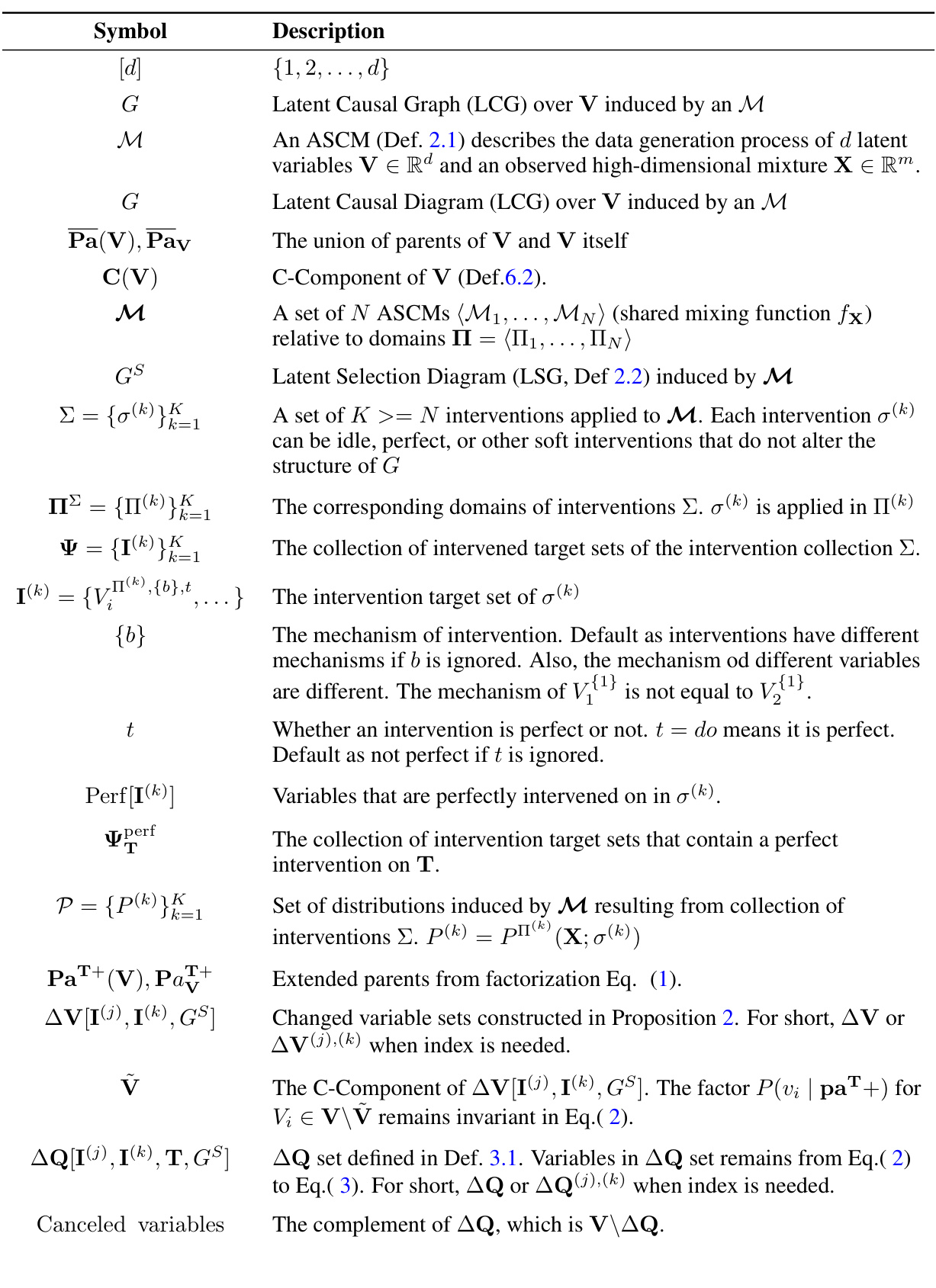
This table compares various works in causal disentangled representation learning. Each row represents a different work, showing its assumptions about the data distribution, the type of interventions allowed, whether it handles multiple domains, and its identifiability results. The assumptions column specifies whether the work assumes a Markovian or non-Markovian causal setting, whether it uses parametric or non-parametric models, and whether it allows for interventions. The data column indicates whether the work uses observational data only, interventional data only, or a combination of both. The identifiability goal column specifies whether the work aims to achieve full disentanglement or a more relaxed version of disentanglement. The output column describes the type of output produced by the algorithm, such as a scaling, mixture, or affine transformation of the latent variables.

This table compares various existing works on causal identifiability in the context of disentangled representation learning. Each row represents a different work, showing the assumptions made (e.g., whether the causal system is Markovian or non-Markovian, whether the distributions are parametric or non-parametric, and whether multiple domains are considered), the type of input data used, and the type of output obtained (e.g., identifiability of the latent variables, or a causal disentanglement map). This table helps to illustrate how the proposed work in the paper builds upon and extends previous work by considering more general assumptions (non-Markovian causal settings, arbitrary distributions from multiple domains), and a more relaxed version of disentanglement.

This table summarizes existing identifiability results in causal representation learning under various assumptions (Markovian/non-Markovian, parametric/non-parametric) and input data (multiple domains, interventions). Each row represents a different study, indicating the assumptions made and the identifiability goals achieved (e.g., full disentanglement, scaling transformations). The table highlights the differences in assumptions and results among various studies and provides context for the current work’s contributions.

This table compares different works in disentangled causal representation learning based on several criteria. These include whether the work handles non-Markovian settings, uses nonparametric distributions, incorporates interventions, and considers multiple domains. The table also notes the assumptions made by each work (e.g., type of distribution, independence assumptions), what type of data was used, the identifiability goal (e.g., full disentanglement, scaling, etc.), and the type of output produced (e.g., functional dependency map, causal disentanglement map). The table shows that this paper is the first to handle non-Markovian settings, arbitrary distributions across multiple domains, and a relaxed version of disentanglement.
Full paper#
