TL;DR#
Deep learning models for survival analysis often prioritize discrimination (ability to differentiate patients with varying risks) over calibration (alignment of predictions with observed event distribution). Ranking losses, commonly used to enhance discrimination, often negatively affect calibration. This leads to clinically less useful predictions, potentially resulting in overtreatment or underestimation of risk.
ConSurv, a novel contrastive learning method, addresses this trade-off. It utilizes informed sampling within a contrastive learning framework, assigning lower penalties to samples with similar survival outcomes. This leverages the intuition that patients with similar event times share similar clinical statuses. Combined with a negative log-likelihood loss, it significantly improves discrimination without directly manipulating model outputs, achieving better calibration. Experiments show ConSurv’s superior performance compared to existing deep survival models in both discrimination and calibration, verified through extensive ablation studies.
Key Takeaways#
Why does it matter?#
This paper is crucial because it tackles a critical issue in survival analysis: the trade-off between discrimination and calibration. By introducing a novel contrastive learning approach, it offers a solution that simultaneously enhances model accuracy and reliability, which is vital for making informed clinical decisions and improving patient outcomes. This work opens doors for further research into contrastive learning techniques within survival analysis and their potential applications in other domains needing reliable and accurate predictive models.
Visual Insights#
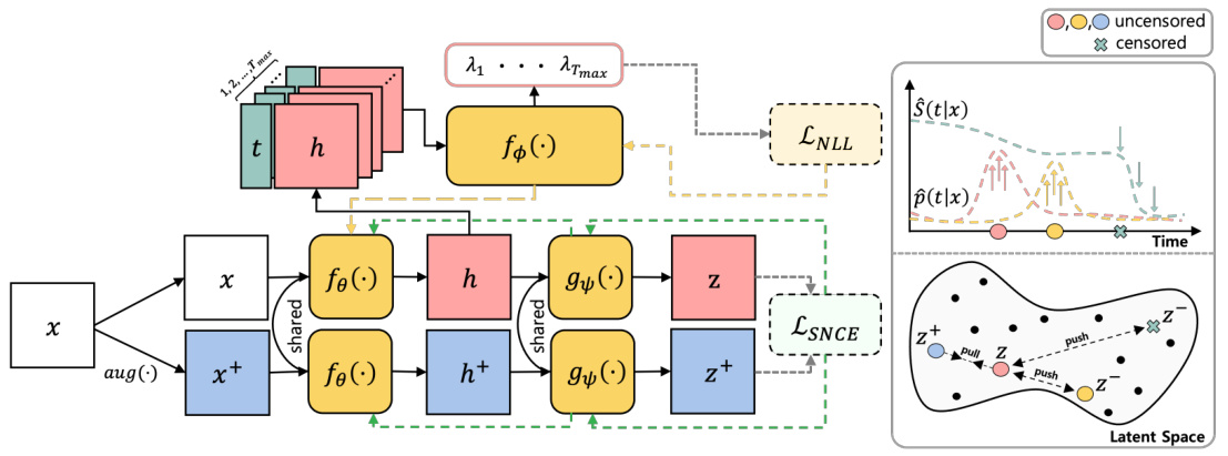
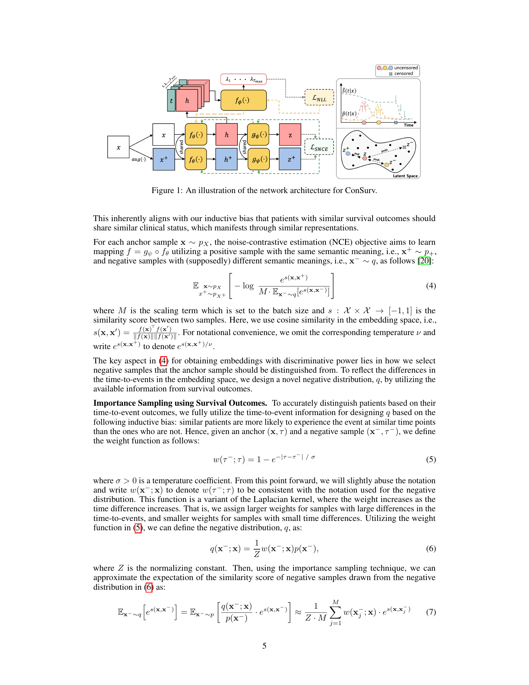
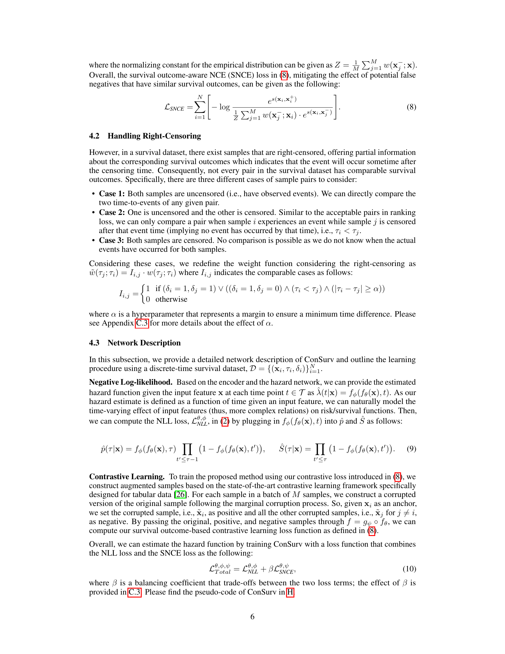
🔼 This figure illustrates the architecture of the ConSurv model, which consists of three main components: an encoder, a projection head, and a hazard network. The encoder takes the input features x and outputs latent representations h. The projection head maps the latent representations to an embedding space where contrastive learning is applied, and the hazard network predicts the hazard rate at each time point t given the latent representation h. The model uses a contrastive learning loss to enhance discrimination while maintaining calibration by incorporating importance sampling based on survival outcomes. The figure also shows how the model handles right-censoring, by assigning lower penalties to potential false negative pairs based on the similarity of their survival outcomes, thus ensuring that samples with similar event times likely share similar clinical statuses.
read the caption
Figure 1: An illustration of the network architecture for ConSurv.
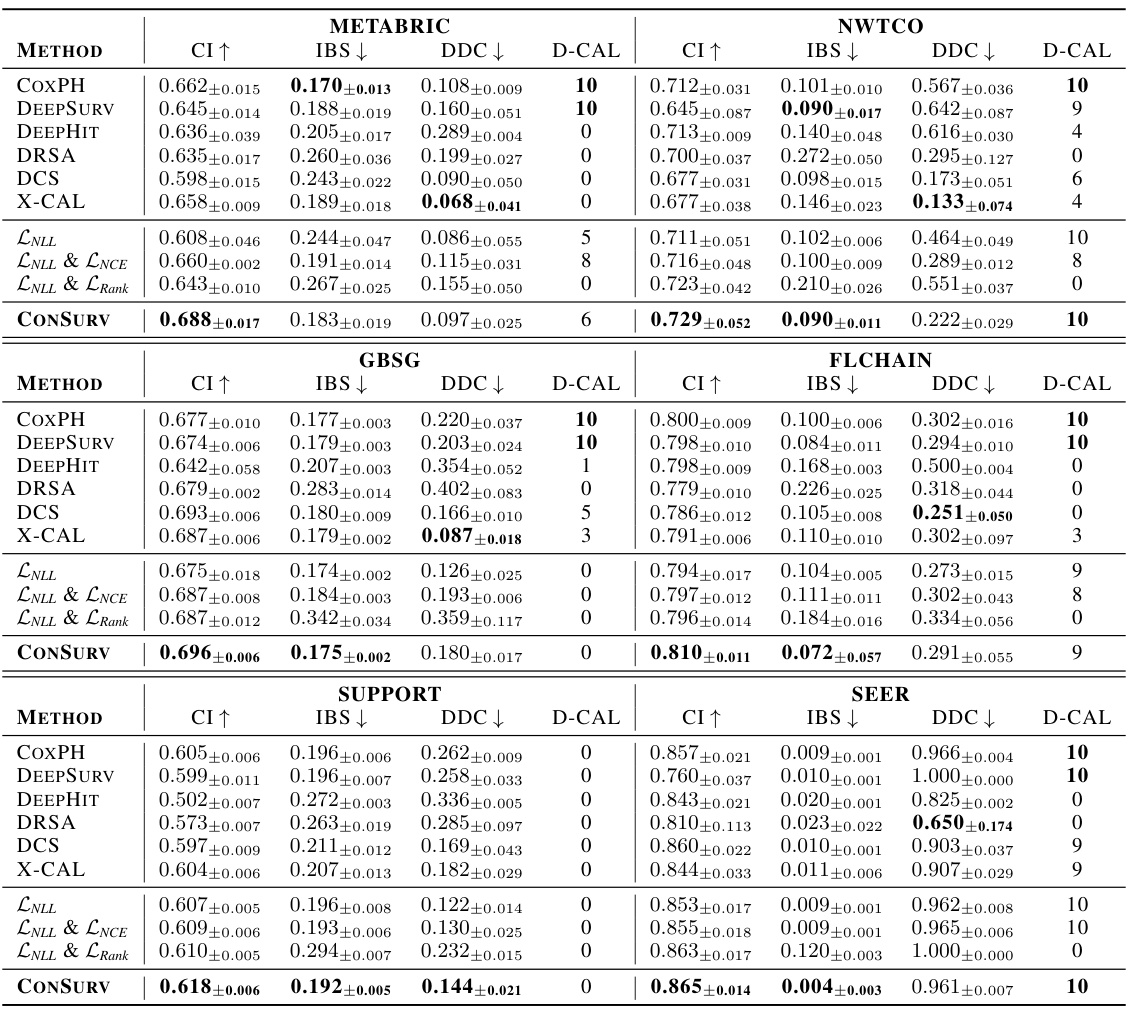
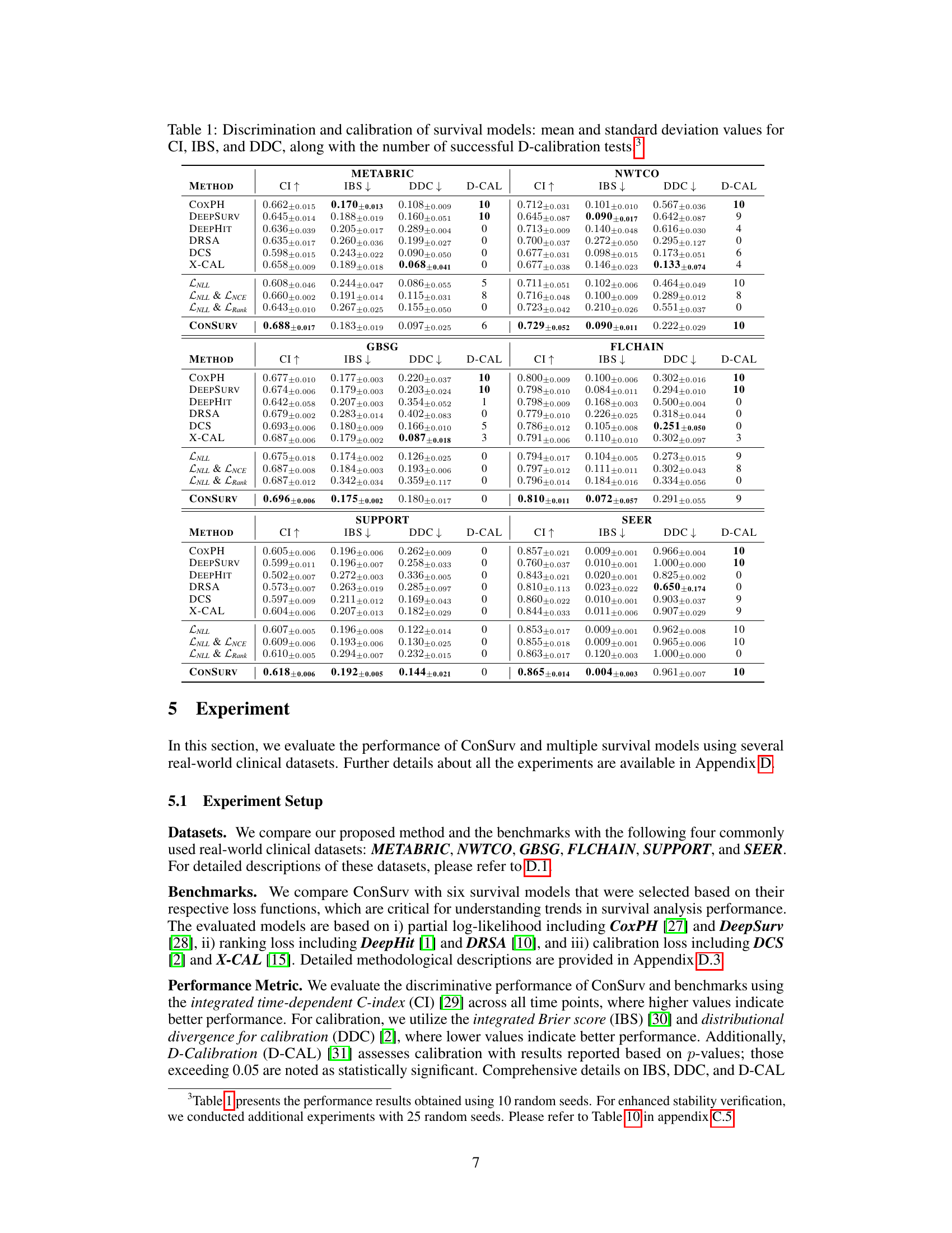
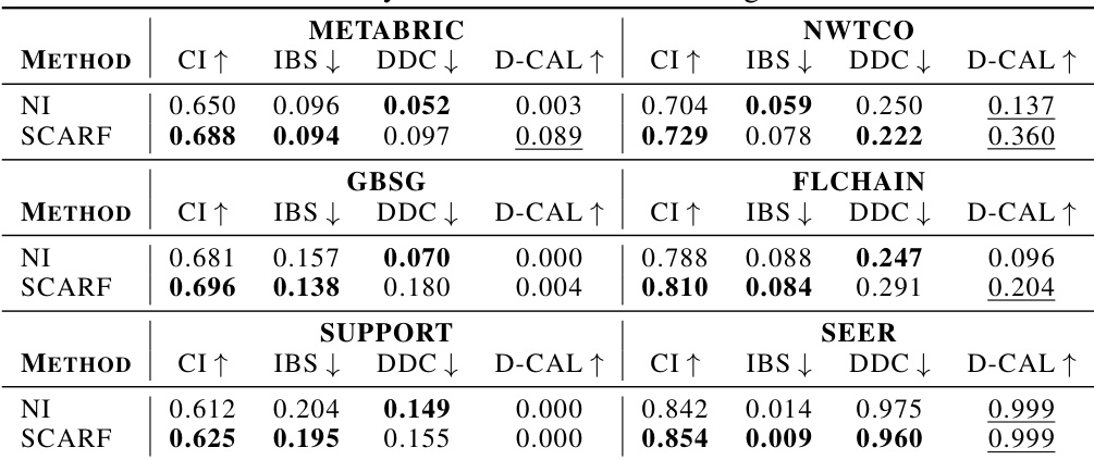
🔼 This table presents the performance of various survival models across different datasets. The metrics used to evaluate the models are the concordance index (CI), integrated Brier score (IBS), and distributional divergence for calibration (DDC). Higher CI values indicate better discrimination, while lower IBS and DDC values indicate better calibration. The ‘D-CAL’ column shows the number of successful D-calibration tests (out of 10), which is a measure of calibration quality.
read the caption
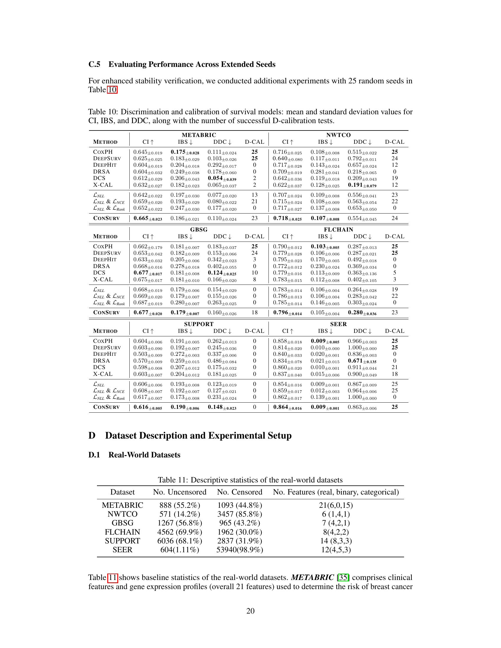
Table 1: Discrimination and calibration of survival models: mean and standard deviation values for CI, IBS, and DDC, along with the number of successful D-calibration tests.
In-depth insights#
Survival Outcome Bias#
Survival outcome bias, in the context of survival analysis, refers to the systematic error introduced when the selection of samples or the assignment of weights is influenced by the knowledge of survival outcomes. This bias can severely compromise the reliability and generalizability of the model, as it may not accurately reflect the true underlying relationships between predictors and survival time. The bias emerges when samples with longer survival times are over-represented, leading to an overly optimistic prediction of survival. Addressing this requires careful consideration of sampling methods and weighting schemes, with a strong emphasis on techniques that avoid preferentially including information about the outcome variable during the data selection or model training phase. Methods like inverse probability of censoring weighting or propensity score matching could potentially mitigate this bias, but careful validation and testing are needed to ensure effectiveness in the specific application. The use of counterfactual methods or methods that directly model the censoring mechanism also show promise in minimizing bias and providing a more robust prediction.
Contrastive Learning#
Contrastive learning, a powerful technique in representation learning, focuses on learning an embedding space where similar data points cluster together while dissimilar points are pushed apart. In the context of survival analysis, this translates to learning a representation that effectively distinguishes between patients with varying survival outcomes. The paper explores how contrastive learning, when augmented with careful sampling strategies, can improve the calibration and discrimination of survival models. By weighting negative samples based on the similarity of their survival outcomes, the method encourages the model to learn meaningful relationships between features and survival time, thereby enhancing both its ability to predict survival time accurately and rank patients effectively. This approach contrasts with traditional ranking-based methods that often prioritize discrimination at the expense of calibration. The key contribution lies in intelligently leveraging the contrastive framework to learn better representations rather than directly manipulating model outputs, addressing a crucial limitation of traditional survival analysis methods. The use of weighted sampling is particularly crucial for handling the complexities of right-censored data inherent in survival analysis, ensuring that the model is not overly influenced by incomplete information.
Calibration Focus#
A focus on calibration in machine learning models, particularly in survival analysis, is critical for ensuring that predicted probabilities accurately reflect real-world outcomes. Poor calibration can lead to misinformed decisions, particularly in high-stakes applications like healthcare, where accurate risk assessment is paramount. Improving calibration often involves using techniques beyond simple discrimination metrics, such as the concordance index (C-index), which primarily assess ranking ability. Methods for improving calibration might involve explicitly incorporating calibration metrics into the loss function during model training, utilizing techniques that directly model the probability distribution of survival times rather than just rankings, or employing advanced calibration methods such as Platt scaling or isotonic regression. The choice of approach will depend on the specific application and the trade-offs between calibration and discrimination performance. Achieving well-calibrated models often requires careful consideration of data characteristics, model architecture, and training techniques. Ultimately, a well-calibrated model is crucial for building trust and ensuring responsible use of machine learning in real-world applications.
Clinical Dataset Tests#
A hypothetical ‘Clinical Dataset Tests’ section in a research paper would likely detail the application of the proposed method (e.g., a new survival analysis model) to multiple real-world clinical datasets. Comprehensive testing is crucial for demonstrating the generalizability and robustness of the method. The section should include descriptions of each dataset, including size, characteristics (e.g., demographics, types of events), and any preprocessing steps taken. Key performance metrics, such as the concordance index (C-index), integrated Brier score (IBS), and calibration metrics should be reported for each dataset, along with statistical significance tests to compare the new method to existing benchmarks. Subgroup analyses might be included to assess performance across different patient subgroups. Visualizations, such as calibration plots and survival curves, would help illustrate the performance of the model and compare it to existing methods. A discussion of any discrepancies or unexpected findings across datasets is important to provide a nuanced and holistic evaluation of the model’s capabilities.
Future Directions#
Future research could explore several promising avenues. Improving the handling of censored data is crucial, as it significantly impacts the accuracy and reliability of survival analysis. This could involve developing novel methods that effectively leverage partial information from censored observations to enhance model performance. Another area of focus should be on developing more robust and generalizable contrastive learning techniques specifically tailored for survival data. Exploring different similarity measures and weighting schemes could improve the efficiency and effectiveness of these methods. Addressing the computational cost of contrastive learning, particularly with large datasets, is important for making these methods more practical in real-world applications. Finally, future work should investigate the application of these techniques in diverse clinical settings, potentially incorporating external data sources or leveraging advanced deep learning architectures like transformers to further improve predictive accuracy and clinical utility.
More visual insights#
More on figures

🔼 This figure displays the t-SNE visualizations of latent representations learned by three different training methods: using only the negative log-likelihood loss (LNLL), using only the survival outcome-aware noise contrastive estimation loss (SNCE), and using both LNLL and SNCE (ConSurv). The visualizations are performed on the METABRIC dataset, and the points are colored according to their event times for better understanding of how different training methods affect the clustering of data points in the latent space.
read the caption
Figure 2: t-SNE visualization for latent representations learned with LNLL only, LSNCE only, and ConSurvfor the METABRIC dataset, colored by event times (for uncensored samples).

🔼 This figure illustrates the network architecture of ConSurv, which consists of three main components: an encoder that maps input features to latent representations, a projection head that maps latent representations to an embedding space for contrastive learning, and a hazard network that predicts the hazard rate at each time point given the latent representation. The contrastive learning part of the network calculates the loss between similar samples (positive pairs) and dissimilar samples (negative pairs) in the embedding space to learn better representations that differentiate patients based on their survival outcomes.
read the caption
Figure 1: An illustration of the network architecture for ConSurv.

🔼 This figure illustrates the network architecture of ConSurv, which consists of three main components: an encoder that maps input features to a latent representation, a projection head that projects the latent representation to an embedding space where contrastive learning is applied, and a hazard network that predicts the hazard rate at each time point given the latent representation. The figure also visually depicts the contrastive learning process within the embedding space, showing how similar samples are pulled together and dissimilar samples are pushed apart. Finally, it shows how the negative log-likelihood (NLL) loss and the survival outcome-aware noise-contrastive estimation (SNCE) loss are combined to train the model.
read the caption
Figure 1: An illustration of the network architecture for ConSurv.
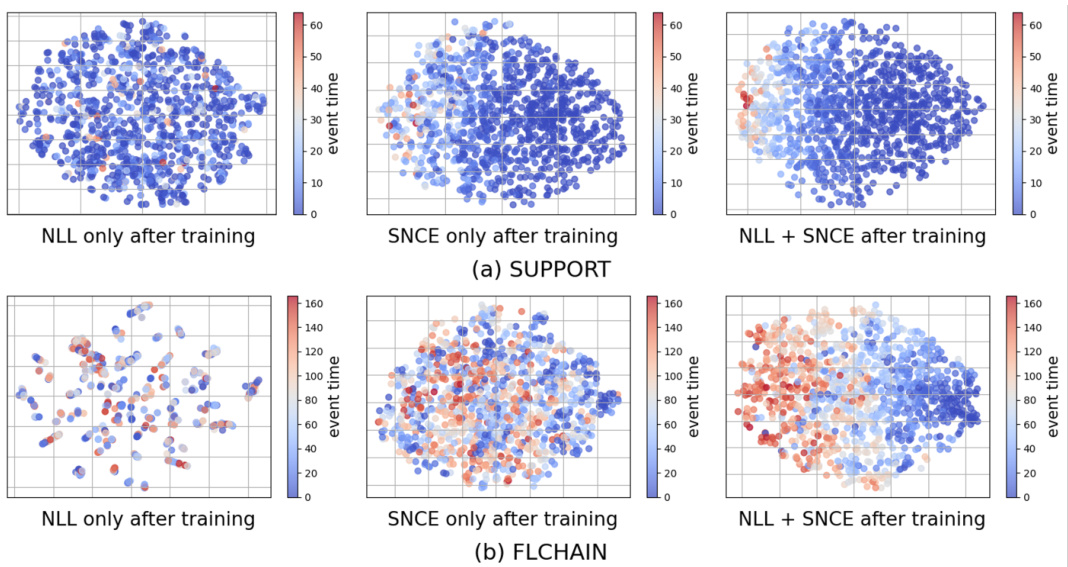
🔼 This figure displays t-SNE visualizations of the latent representations learned by three different training methods: using only the negative log-likelihood (NLL) loss, using only the survival outcome-aware noise contrastive estimation (SNCE) loss, and using both NLL and SNCE losses (ConSurv). The visualizations are performed on the METABRIC dataset and colored according to the event times of uncensored samples. This allows for a visual comparison of how well each method separates samples based on their survival outcomes in the latent space. The goal is to demonstrate that ConSurv effectively captures and reflects the underlying event time information to improve the model’s discrimination.
read the caption
Figure 2: t-SNE visualization for latent representations learned with LNLL only, LSNCE only, and ConSurv for the METABRIC dataset, colored by event times (for uncensored samples).
🔼 The figure illustrates the network architecture of the proposed ConSurv model for survival analysis. It shows the encoder, projection head, and hazard network, along with the contrastive learning and negative log-likelihood loss components. The data flow is visualized, starting with input features and culminating in hazard predictions in the latent space. This visualization helps to understand how the model processes input data and produces its predictions by contrasting samples based on their survival times to improve calibration, while using maximum likelihood estimation to preserve it.
read the caption
Figure 1: An illustration of the network architecture for ConSurv.
🔼 This figure illustrates the network architecture of ConSurv, which consists of three main components: an encoder that maps input features to latent representations, a projection head that maps latent representations to an embedding space where contrastive learning is applied, and a hazard network that predicts the hazard rate at each time point given the latent representation. The figure also shows how the components are connected, and how the output of the hazard network is used for maximum likelihood estimation (MLE).
read the caption
Figure 1: An illustration of the network architecture for ConSurv.

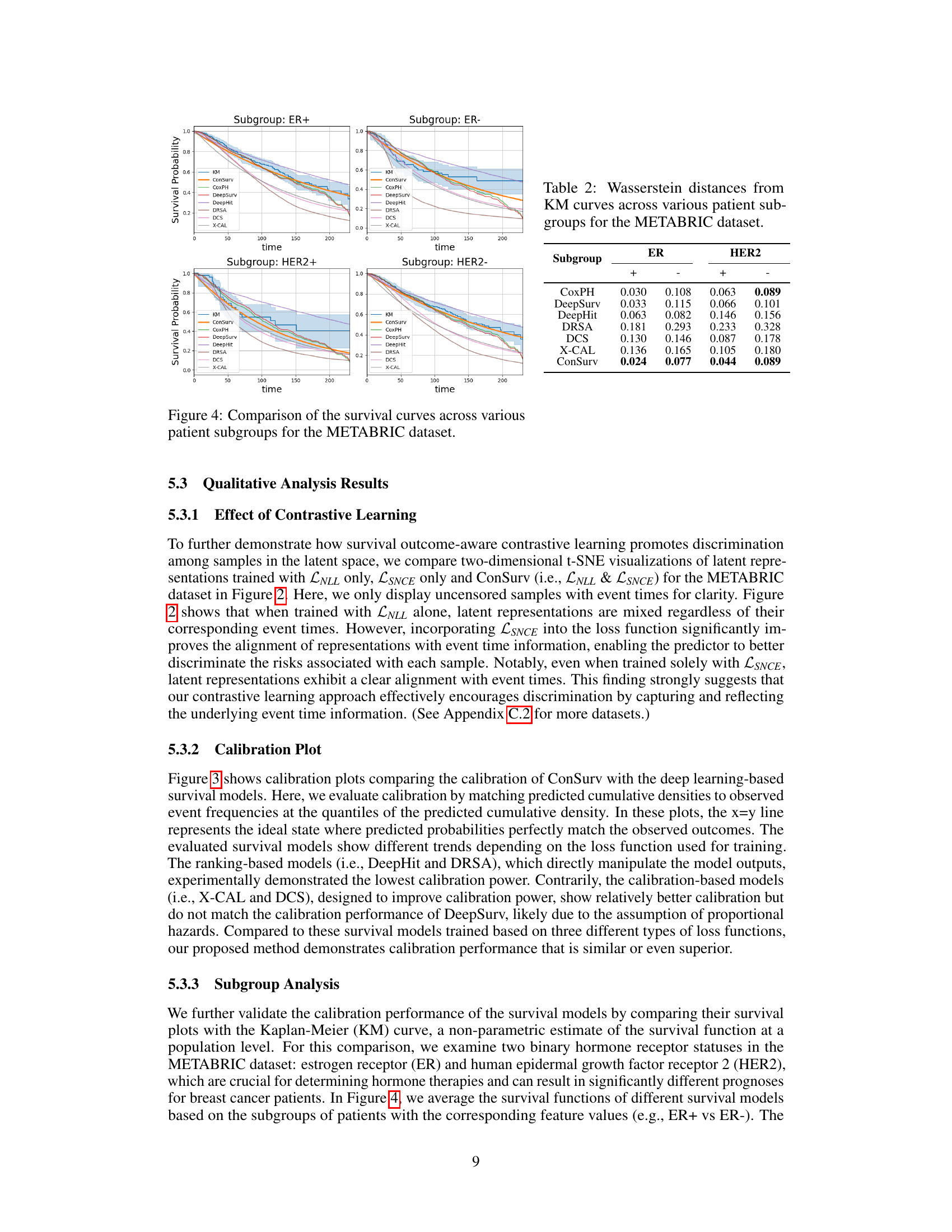
🔼 This figure compares the survival curves predicted by ConSurv and other benchmark models against the Kaplan-Meier (KM) curve for three different subgroups of patients in the METABRIC dataset based on cellularity. Each plot visualizes the survival probability over time for each model and the KM curve, highlighting the differences in survival outcomes across these subgroups.
read the caption
Figure 8: Comparison of the survival curves across various patient subgroups in the METABRIC dataset.

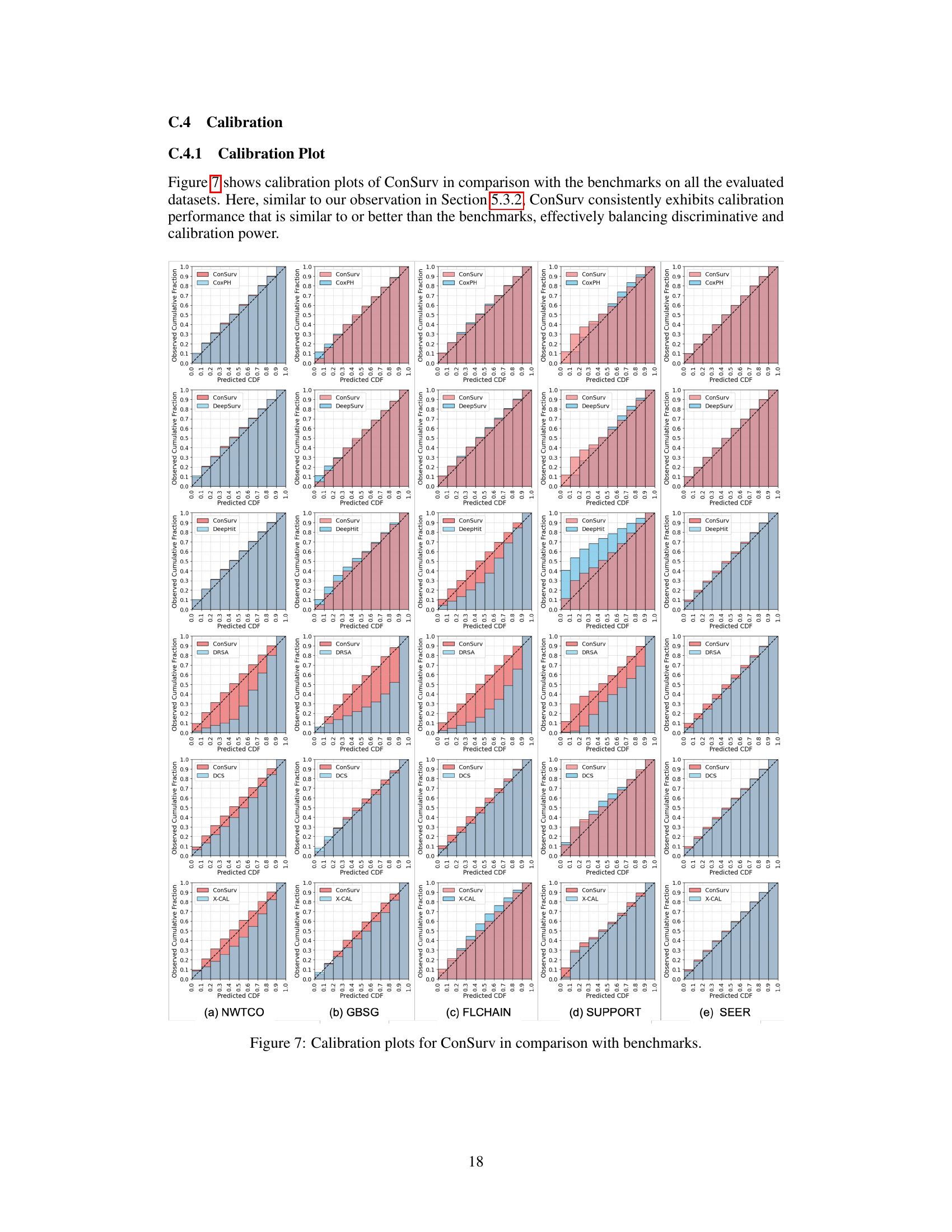
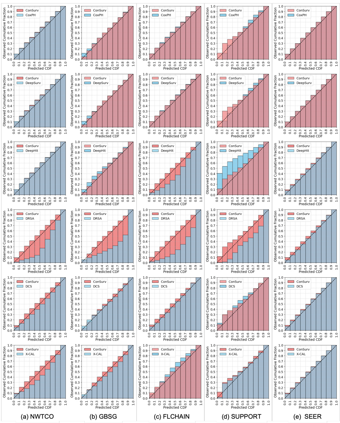
🔼 This figure presents calibration plots that compare the performance of the proposed ConSurv model against several benchmark models on the METABRIC dataset. Calibration plots assess how well a model’s predicted probabilities align with observed outcomes. Each plot shows the predicted cumulative distribution function (CDF) against the observed cumulative fraction. A perfectly calibrated model would have its points fall along the diagonal line (x=y), indicating perfect alignment between predictions and observations. Deviations from this diagonal suggest miscalibration. The plots allow for a visual comparison of the calibration performance between ConSurv and other approaches, illustrating the relative strengths and weaknesses in accurately predicting survival probabilities.
read the caption
Figure 3: Calibration plots for ConSurv in comparison with benchmarks for the METABRIC dataset.
More on tables

🔼 This table presents the performance comparison of different survival models across multiple datasets. The models’ performance is evaluated using three key metrics: Concordance Index (CI), Integrated Brier Score (IBS), and Distributional Divergence for Calibration (DDC). Higher CI values indicate better discrimination ability, while lower IBS and DDC values indicate better calibration. The number of successful D-calibration tests is also reported, which is a statistical test for assessing calibration quality. The table allows for a comprehensive assessment of both the discrimination and calibration capabilities of various survival models.
read the caption
Table 1: Discrimination and calibration of survival models: mean and standard deviation values for CI, IBS, and DDC, along with the number of successful D-calibration tests.
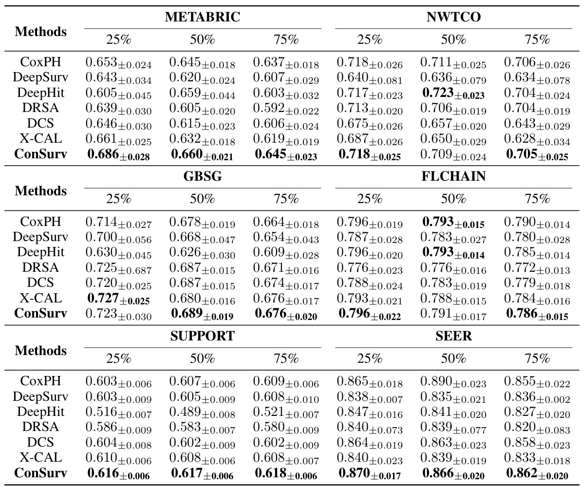
🔼 This table presents the performance of various survival models (ConSurv and benchmarks) across four real-world datasets (METABRIC, NWTCO, GBSG, FLCHAIN). For each model and dataset, it shows the mean and standard deviation of three key metrics: the concordance index (CI), which measures discrimination ability; the integrated Brier score (IBS), which measures calibration; and the distributional divergence for calibration (DDC), another calibration metric. It also indicates the number of times the D-calibration test, a statistical test for calibration, yielded a p-value above 0.05 (D-CAL), suggesting successful calibration.
read the caption
Table 1: Discrimination and calibration of survival models: mean and standard deviation values for CI, IBS, and DDC, along with the number of successful D-calibration tests.
🔼 This table presents the performance evaluation results of various survival models on four benchmark datasets. For each model and dataset, it shows the mean and standard deviation of the concordance index (CI), integrated Brier score (IBS), and distributional divergence for calibration (DDC). It also indicates how many times (out of ten) the D-calibration test showed statistically significant results, providing insights into the calibration quality of the models.
read the caption
Table 1: Discrimination and calibration of survival models: mean and standard deviation values for CI, IBS, and DDC, along with the number of successful D-calibration tests.

🔼 This table presents the results of comparing ConSurv with six other survival models across four different datasets. For each model and dataset, it shows the mean and standard deviation of three evaluation metrics: the concordance index (CI), integrated Brier score (IBS), and distributional divergence for calibration (DDC). Additionally, it provides the number of times that the D-calibration test (a measure of calibration quality) resulted in a p-value exceeding 0.05 (indicating acceptable calibration). This allows for a comparison of the models’ performance in both discrimination and calibration.
read the caption
Table 1: Discrimination and calibration of survival models: mean and standard deviation values for CI, IBS, and DDC, along with the number of successful D-calibration tests.
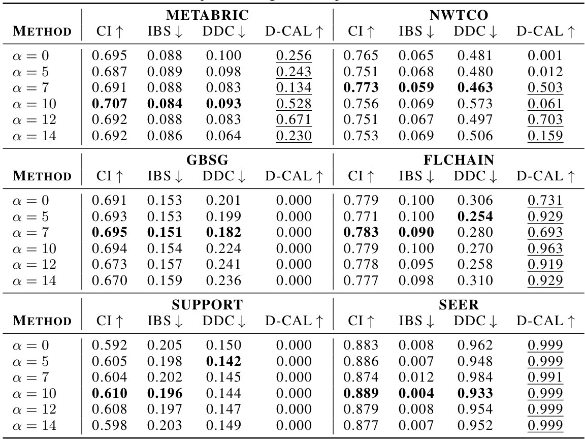
🔼 This table presents the performance of different survival models on four benchmark datasets. For each model and dataset, it shows the mean and standard deviation of three key metrics: the concordance index (CI), which measures discrimination; the integrated Brier score (IBS), which measures calibration; and the distributional divergence for calibration (DDC), another calibration metric. It also indicates how many out of ten D-calibration tests (a calibration test) were successful for each model.
read the caption
Table 1: Discrimination and calibration of survival models: mean and standard deviation values for CI, IBS, and DDC, along with the number of successful D-calibration tests.

🔼 This table presents the performance of several survival models across multiple datasets. For each model and dataset, it shows the mean and standard deviation of three metrics: Concordance Index (CI), Integrated Brier Score (IBS), and Distributional Calibration Divergence (DDC). Higher CI values indicate better discrimination, while lower IBS and DDC values signify better calibration. The ‘D-CAL’ column indicates how many out of ten D-calibration tests were statistically significant (p-value > 0.05).
read the caption
Table 1: Discrimination and calibration of survival models: mean and standard deviation values for CI, IBS, and DDC, along with the number of successful D-calibration tests.
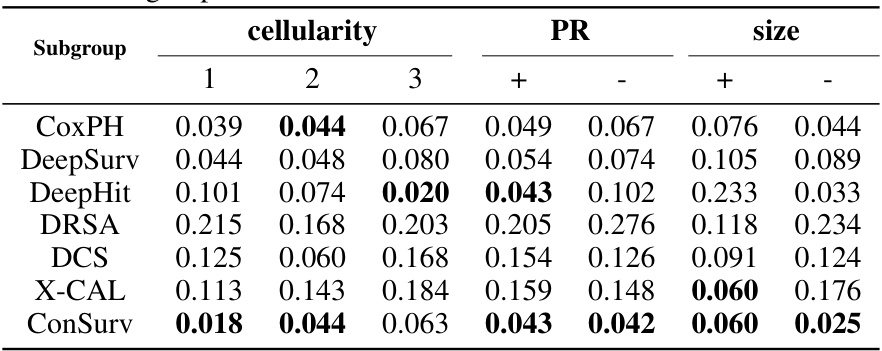
🔼 This table presents the performance of various survival models (including ConSurv) across four different datasets. For each model and dataset, the table shows the mean and standard deviation of three key metrics: the concordance index (CI, measuring discrimination), the integrated Brier score (IBS, measuring calibration), and the distributional calibration divergence (DDC, another measure of calibration). The number of successful D-calibration tests (D-CAL) is also reported, indicating the statistical significance of calibration performance.
read the caption
Table 1: Discrimination and calibration of survival models: mean and standard deviation values for CI, IBS, and DDC, along with the number of successful D-calibration tests.
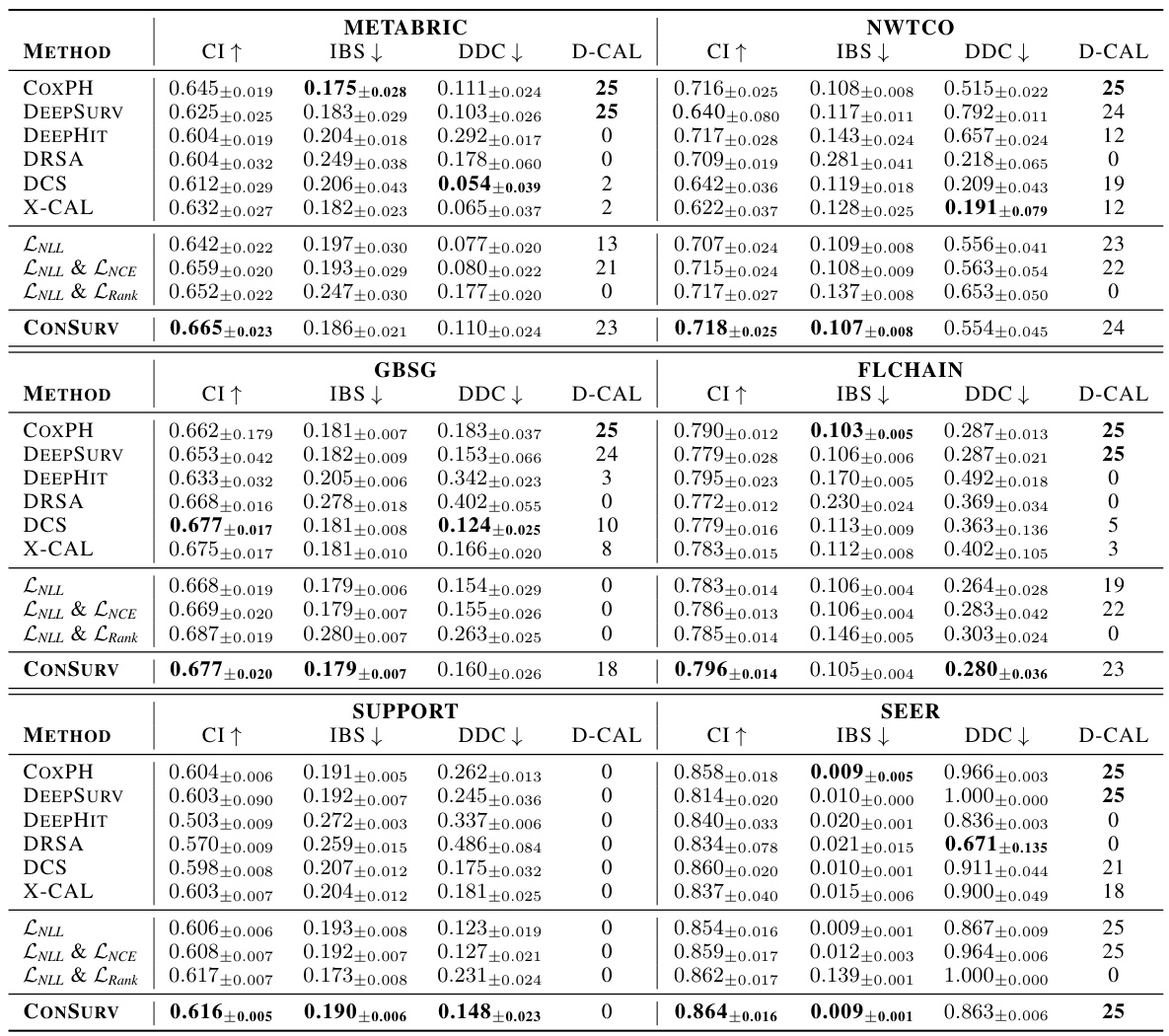
🔼 This table presents the performance of various survival models across four different datasets. The models’ discrimination performance is evaluated using the concordance index (CI), while calibration is assessed using the integrated Brier score (IBS) and the distributional divergence for calibration (DDC). The number of successful D-calibration tests is also reported for each model and dataset. Higher CI values and lower IBS/DDC values indicate better model performance. The table serves as a key comparison for the proposed ConSurv model against existing benchmarks.
read the caption
Table 1: Discrimination and calibration of survival models: mean and standard deviation values for CI, IBS, and DDC, along with the number of successful D-calibration tests.

🔼 This table presents the performance of various survival models across multiple datasets. The metrics used are the concordance index (CI), integrated Brier score (IBS), and distributional divergence for calibration (DDC). Higher CI values indicate better discrimination, while lower IBS and DDC values indicate better calibration. The ‘D-CAL’ column shows the number of times the D-calibration test (a measure of calibration) produced a p-value above 0.05 (indicating successful calibration). The table compares the performance of ConSurv to several benchmark models, allowing for a comprehensive assessment of both discrimination and calibration.
read the caption
Table 1: Discrimination and calibration of survival models: mean and standard deviation values for CI, IBS, and DDC, along with the number of successful D-calibration tests.

🔼 This table presents the performance of various survival models across multiple datasets. For each model and dataset, it shows the mean and standard deviation of three key metrics: concordance index (CI), integrated Brier score (IBS), and distributional divergence for calibration (DDC). A higher CI indicates better discrimination, while lower IBS and DDC values indicate better calibration. Finally, it also includes the number of times (out of 10 trials) that the model passed the D-calibration test, demonstrating its calibration ability.
read the caption
Table 1: Discrimination and calibration of survival models: mean and standard deviation values for CI, IBS, and DDC, along with the number of successful D-calibration tests.
Full paper#
