↗ OpenReview ↗ NeurIPS Homepage ↗ Chat
TL;DR#
Simulating light propagation in complex photonic devices is computationally expensive, hindering design and optimization. Existing neural network approaches struggle to achieve high accuracy, especially for intricate devices with complex light-matter interactions.
The researchers propose PACE, a novel neural operator with a cross-axis factorized architecture. PACE’s design is inspired by human learning, employing a two-stage training process for high-fidelity results. Experiments show PACE achieves 73% lower error and 50% fewer parameters than existing methods, alongside significant speed improvements over traditional numerical solvers. This work demonstrates a major advance in accurate and efficient optical field simulation, boosting the photonic circuit design process.
Key Takeaways#
Why does it matter?#
This paper is crucial for researchers in photonics and machine learning because it significantly advances the accuracy and speed of optical field simulation. Its novel PACE operator and two-stage learning framework offer a powerful approach to overcome challenges in simulating complex photonic devices. This opens avenues for faster design cycles, improved device optimization, and accelerates progress in integrated photonics.
Visual Insights#

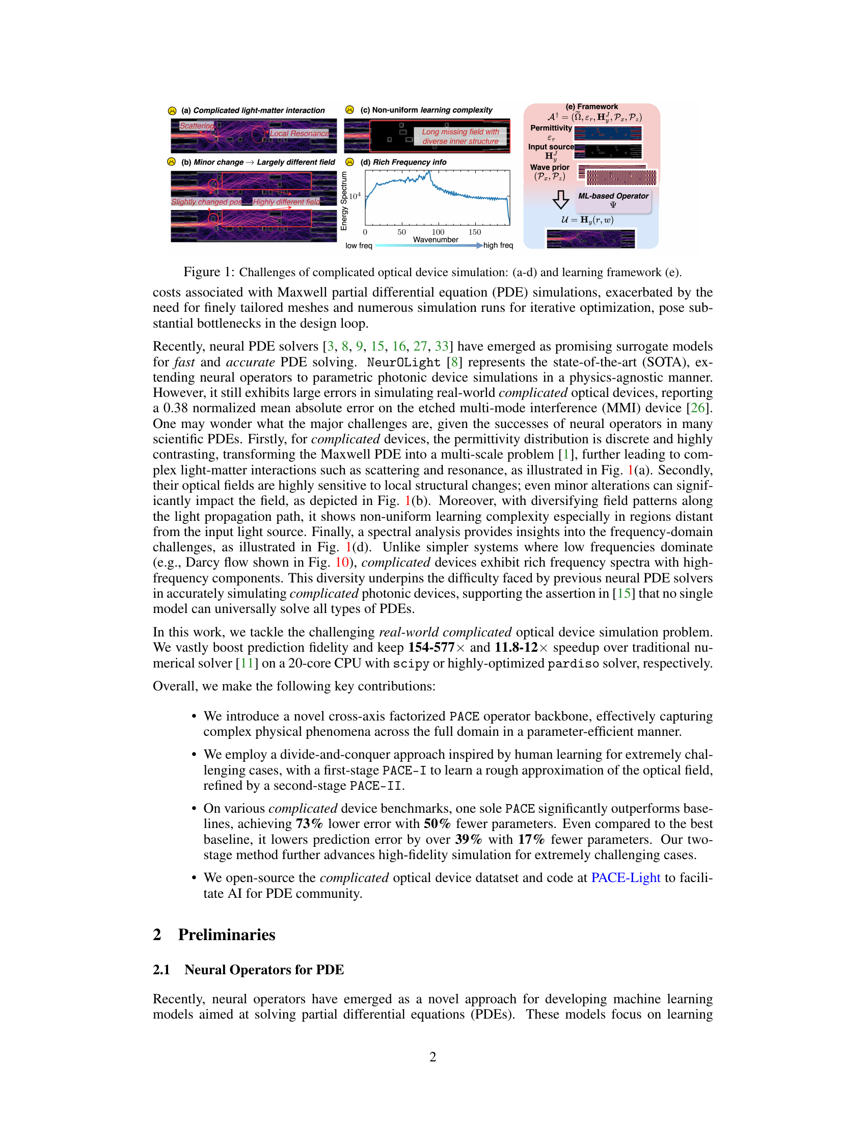
This figure illustrates the challenges in simulating complicated optical devices and the proposed learning framework. (a) shows the complex interplay of light and matter, including scattering and resonance effects. (b) highlights the sensitivity of the optical field to minor changes in device structure. (c) demonstrates the non-uniform learning complexity across the simulation domain, with more challenging regions farther from the light source. (d) presents the rich frequency spectrum of the optical field, a factor that makes accurate prediction difficult. Finally, (e) shows the learning framework, which takes the permittivity distribution, input light source, and wave priors as input and predicts the optical field.

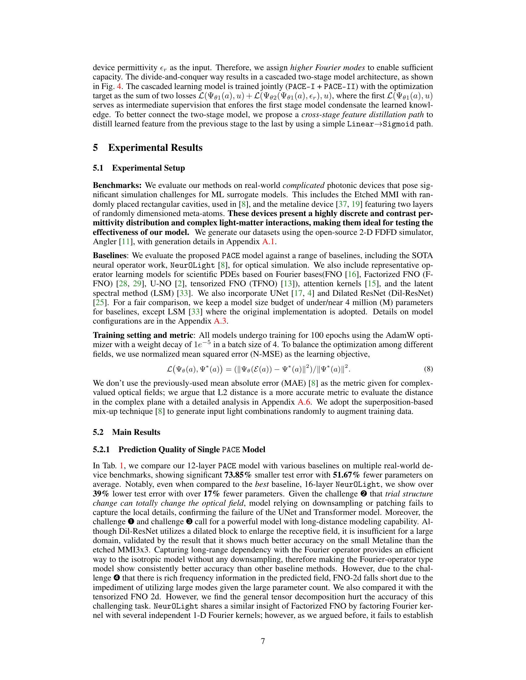
This table compares the performance of the proposed PACE model against various baselines on three real-world complicated photonic device benchmarks. The metrics used for comparison include the number of parameters (#Params), training error (Train Err), and test error (Test Err). The table shows that PACE significantly outperforms existing methods in terms of lower error and fewer parameters. Overall improvements across all benchmarks are summarized using geometric means.
In-depth insights#
PACE Operator Design#
The core of the research lies in the innovative design of the PACE (Pacing Operator) for accurate and efficient optical field simulation. PACE leverages a cross-axis factorized integral kernel, enabling it to effectively capture long-range dependencies and relationships between local device structures and the global optical field. This design addresses limitations of previous neural operators which struggled with capturing complex light-matter interactions and high-frequency components in real-world, intricate photonic devices. The incorporation of a self-weighted path enhances the operator’s ability to focus attention on locally significant features, while an explicit projection unit aids in capturing high-frequency information. The combination of these design choices leads to superior performance compared to existing state-of-the-art methods, demonstrating a significant reduction in prediction error and a substantial increase in computational speed.
Cascaded Learning#
The proposed “Cascaded Learning” approach is a novel two-stage training strategy that mimics human learning. Instead of directly tackling a complex optical field simulation problem, it breaks it down into two progressively simpler tasks. Stage one uses a model (PACE-I) to learn a rough initial solution based on readily available information like the light source and permittivity distribution. Stage two then employs a second model (PACE-II) to refine this initial estimate, leveraging the previous stage’s output as input along with additional data. This divide-and-conquer strategy is particularly effective for extremely difficult simulation scenarios that would otherwise overwhelm a single model. Cross-stage feature distillation is employed to seamlessly transfer crucial knowledge from the first stage to the second, enhancing prediction fidelity. The two-stage setup shows a remarkable improvement in accuracy, surpassing a single-stage approach with significantly more layers, highlighting the efficiency and effectiveness of the cascaded learning method for high-fidelity simulations.
High-Fidelity Results#
A section titled ‘High-Fidelity Results’ in a research paper would ideally present a detailed analysis demonstrating the accuracy and precision of the methods or models presented. It should go beyond simply stating high accuracy; instead, it would provide quantitative metrics such as mean absolute error, mean squared error, or other relevant statistical measures, comparing them to existing state-of-the-art methods. Visualizations, such as plots or images showing the model’s output compared to ground truth, would be essential for demonstrating high fidelity. The section would need to address the challenges of achieving high fidelity within the specific context of the research, and how the presented work overcomes those challenges. Furthermore, the robustness of the high-fidelity results, across various inputs or conditions, needs to be explored and presented. Finally, a discussion of the trade-offs between accuracy and computational cost or other relevant factors is important. Without these elements, a ‘High-Fidelity Results’ section would lack the depth and persuasiveness necessary to support the paper’s conclusions.
Computational Speedup#
The research demonstrates a significant computational speedup achieved by the proposed PACE model compared to traditional numerical solvers. This acceleration is crucial for practical applications, especially in the design and optimization of photonic devices, where iterative simulations are often computationally expensive. Speedups ranging from 154x to 577x are reported when using scipy, and 11.8x to 12x when using the highly-optimized pardiso solver. This substantial improvement in efficiency stems from the model’s ability to learn the underlying physics of light propagation and device interactions, allowing it to produce accurate results much faster than traditional methods which rely on computationally intensive numerical approximations. The efficiency gains are further enhanced by the model’s design and the two-stage learning approach used for complex simulations, allowing for more accurate and computationally efficient simulations. The parameter efficiency of PACE is also noteworthy, which is beneficial for deployment on resource-constrained devices.
Future Work#
Future research directions stemming from this work could explore extending PACE to three-dimensional simulations, a significant challenge due to increased computational costs. Addressing this would broaden the applicability of PACE to more complex and realistic photonic devices. Another avenue involves investigating the applicability of PACE to other types of PDEs. While this study focused on Maxwell’s equations for optical field simulation, the underlying principles of PACE’s cross-axis factorization and cascaded learning might prove valuable in solving other physics-based problems. Furthermore, exploring different neural operator architectures or combining PACE with other techniques could lead to further improvements in accuracy and efficiency. Exploring the potential of different numerical methods for solving the underlying PDE, beyond the FDFD method used in this study, could be beneficial. Finally, a deeper investigation into the theoretical foundations of PACE would strengthen our understanding of its success and pave the way for more sophisticated model designs.
More visual insights#
More on figures

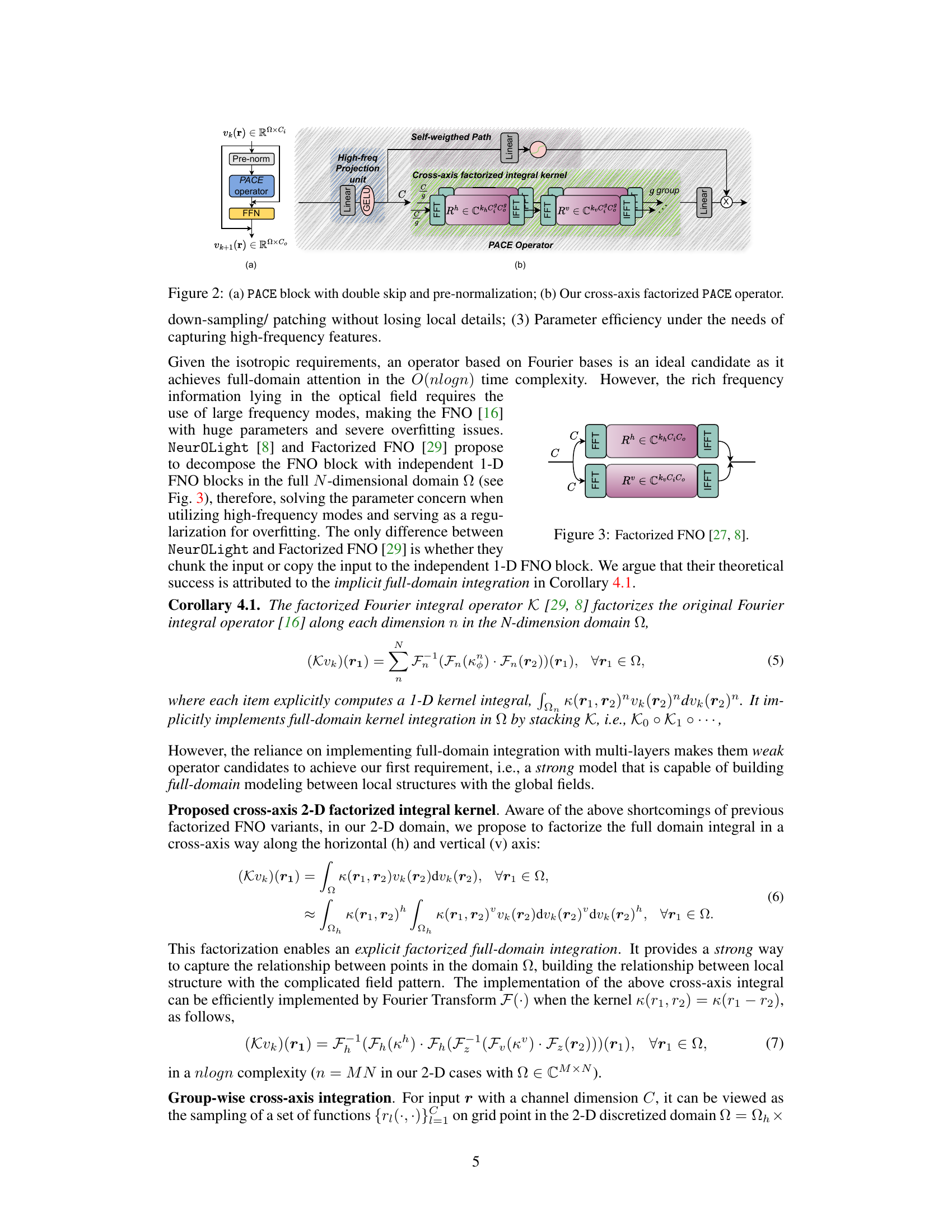
Figure 2(a) shows the PACE block architecture, which includes a pre-normalization step, a PACE operator, a feedforward neural network (FFN), and double skip connections for improved stability and performance in deeper networks. Figure 2(b) details the cross-axis factorized PACE operator, which is the core of the proposed method. It consists of a high-frequency projection unit, a self-weighted path, and a cross-axis factorized integral kernel. The cross-axis factorized integral kernel splits the input into groups and applies a 2D factorization to improve efficiency and better capture long-range dependencies. The figure highlights the key components of the proposed PACE operator and how they work together.

Figure 2(a) shows the PACE block architecture which includes a pre-normalization layer, a PACE operator, a feed-forward network (FFN), and skip connections. Figure 2(b) details the cross-axis factorized PACE operator, highlighting its components: self-weighted paths, high-frequency projection units, and the cross-axis factorized integral kernel. This operator design is crucial to the model’s ability to efficiently capture complex physical phenomena across the full domain and handle high-frequency features in optical field simulations.

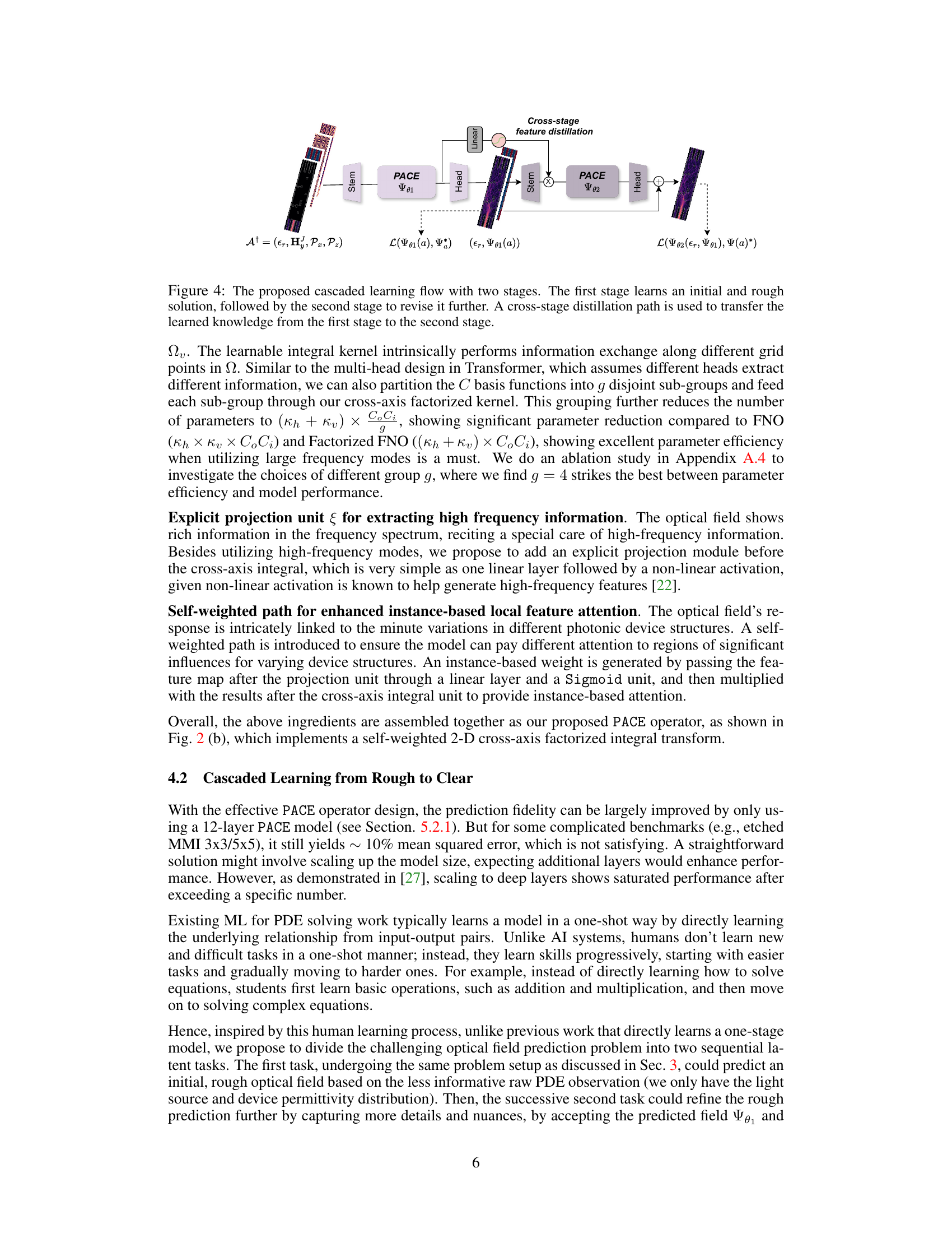
This figure illustrates the two-stage learning process used in the PACE model. The first stage (PACE-I) produces a rough initial solution, which is then refined by the second stage (PACE-II). A cross-stage feature distillation path helps transfer knowledge from the first stage to improve the accuracy of the second stage.

This figure shows the speedup achieved by the PACE model compared to the Angler software, which uses either scipy or pardiso linear solvers for solving the Maxwell PDE. The speedup is presented for different simulation domain sizes, using two different grid step sizes (0.05 nm and 0.075 nm). The results indicate that PACE offers significant speed improvements, particularly for larger simulation domains. The speedup is higher when using the scipy solver compared to the pardiso solver.

This figure shows the generalization ability of the PACE model to unseen wavelengths. The x-axis represents the wavelength (in μm), and the y-axis shows the test normalized mean squared error (N-MSE). The blue stars indicate wavelengths that were present in the training data, while the green plus signs show wavelengths that were not seen during training. The shaded region shows the standard deviation. The figure demonstrates that PACE generalizes well within the C-band (1.53-1.565 μm), a common range for optical communication, and maintains relatively good accuracy even outside of this range, although the error increases with distance from the training wavelengths.

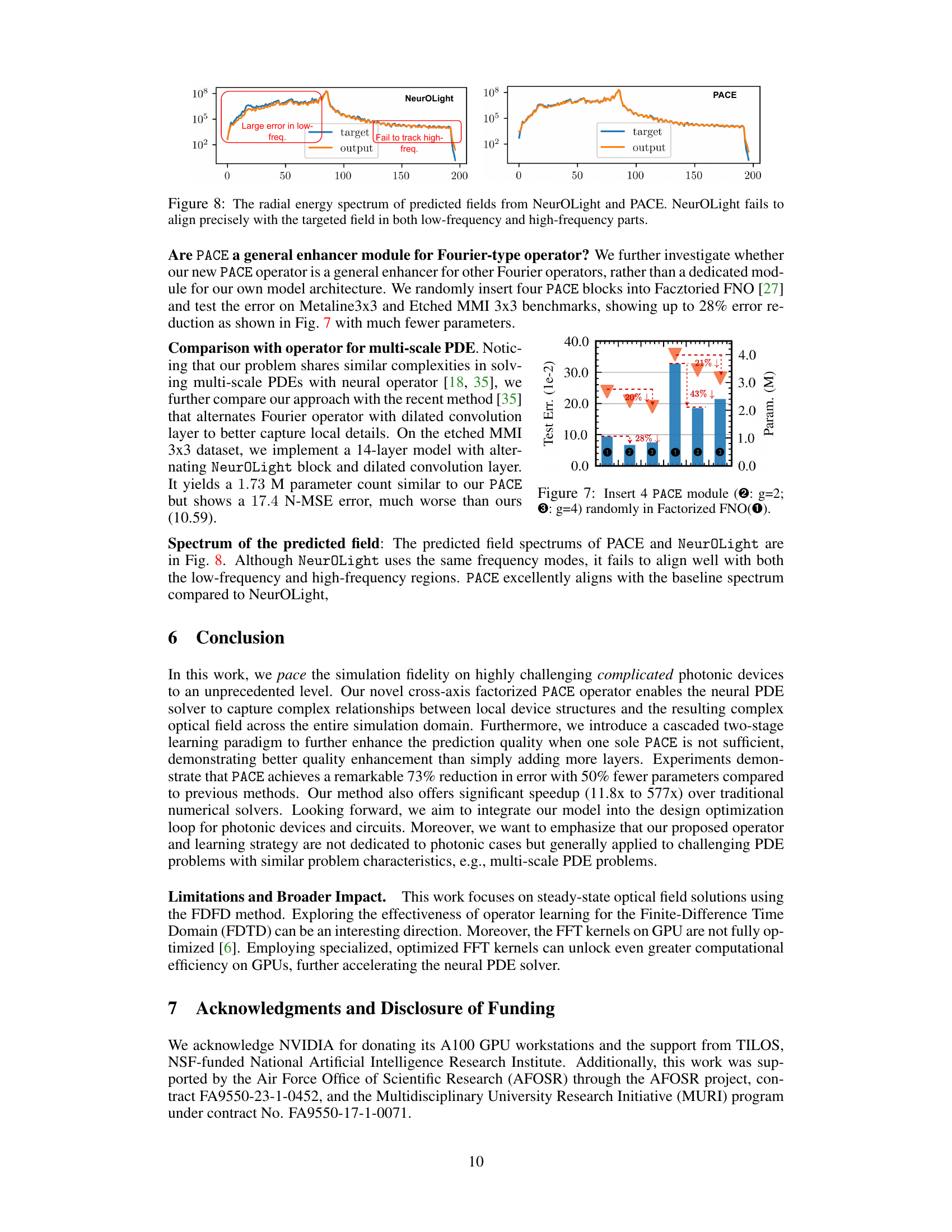
This figure compares the radial energy spectrums of the predicted optical fields from the NeuroLight and PACE models against the ground truth. The plots show the energy distribution as a function of wavenumber (frequency). NeuroLight shows significant errors in both low and high-frequency regions, failing to accurately capture the energy distribution of the target field. In contrast, PACE demonstrates far better alignment with the target spectrum across all frequencies, indicating a superior prediction accuracy.

This figure demonstrates the effectiveness of integrating PACE modules into a pre-existing Factorized Fourier Neural Operator (FNO) model. Three variations of the FNO model are compared: the baseline FNO (①), an FNO with four PACE modules where each module uses a group size of 2 (②), and an FNO with four PACE modules where each module uses a group size of 4 (③). The bar chart shows the test error (y-axis) and the number of parameters (M, second y-axis). The results show that the addition of PACE modules significantly reduces the test error, particularly when using a group size of 4 (③), which demonstrates a 43% decrease in test error compared to the baseline FNO, even with slightly fewer parameters. This highlights PACE’s potential as a general enhancement module for other Fourier-based neural operators, improving their performance without substantial increases in complexity.
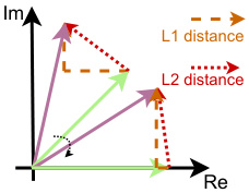
This figure illustrates the difference between L1 and L2 distances in the complex plane. Two complex numbers are represented as vectors from the origin. The L1 distance is the sum of the absolute differences of the real and imaginary components (the length of the dashed brown line), while the L2 distance (Euclidean distance) is the straight-line distance between the two points (the length of the dashed red line). The figure shows that rotating the vectors changes the L1 distance but not the L2 distance, illustrating the rotation invariance of the L2 distance which makes it a better choice for measuring proximity in the complex plane, as the magnitude and angle between complex numbers are both important factors in evaluating similarity.

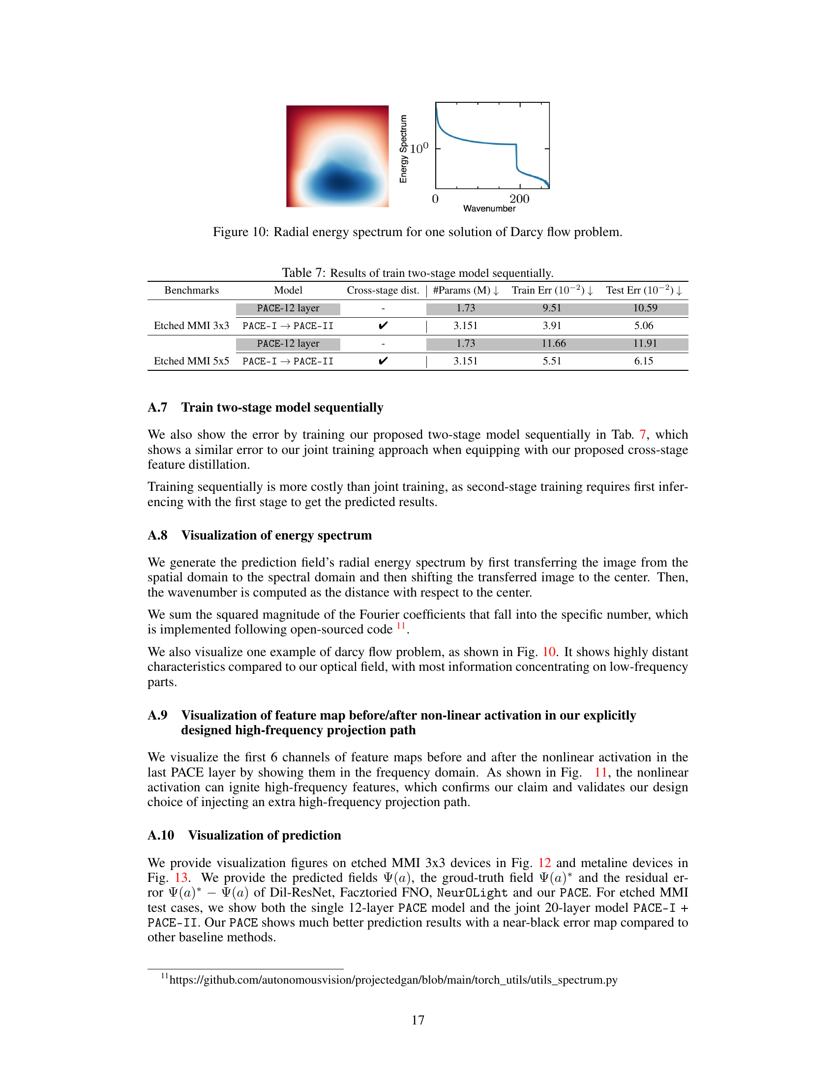
The figure shows a comparison between the spatial representation of a solution to the Darcy flow problem and its corresponding energy spectrum. The spatial representation is a 2D heatmap, where color intensity represents the magnitude of the solution. The energy spectrum is a 1D plot showing the distribution of energy across different spatial frequencies (wavenumbers). The plot shows that most of the energy is concentrated at low wavenumbers, indicating that the solution is dominated by low-frequency components. This contrasts with optical fields in photonic devices, which have rich frequency information.

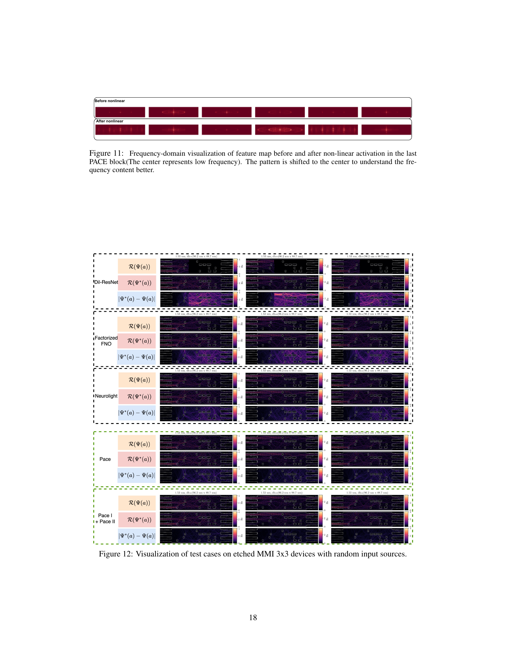
This figure shows the frequency-domain visualization of feature maps before and after applying a non-linear activation function within the high-frequency projection path of the PACE block. The central area of each image represents the low frequencies, and the pattern shift helps to better understand the frequency content of the features. The visualization demonstrates the effect of the non-linear activation in amplifying the high-frequency components.

This figure visualizes the results of several test cases on etched MMI 3x3 devices using various models: Dil-ResNet, Factorized FNO, NeuroLight, and PACE (both single and two-stage). For each model and input source, it shows the real part of the predicted field (R(Ψ(a))), the real part of the ground truth field (R(Ψ*(a))), and the residual error between the prediction and the ground truth (|Ψ*(α) – Ψ(α)|). The visualization provides a qualitative comparison of the different models’ performance in capturing the complex optical field patterns in the etched MMI devices.

This figure visualizes the results of several test cases on etched MMI 3x3 devices. For each test case, it shows the real part of the predicted optical field (R(Ψ(α))), the real part of the ground-truth optical field (R(Ψ*(α))), and the difference between them (R(Ψ*(α))−R(Ψ(α))). The models compared include Dil-ResNet, Factorized FNO, NeuroLight, and the proposed PACE model. The figure demonstrates the superior accuracy of the PACE model compared to the baselines in predicting the optical field for these devices.
More on tables

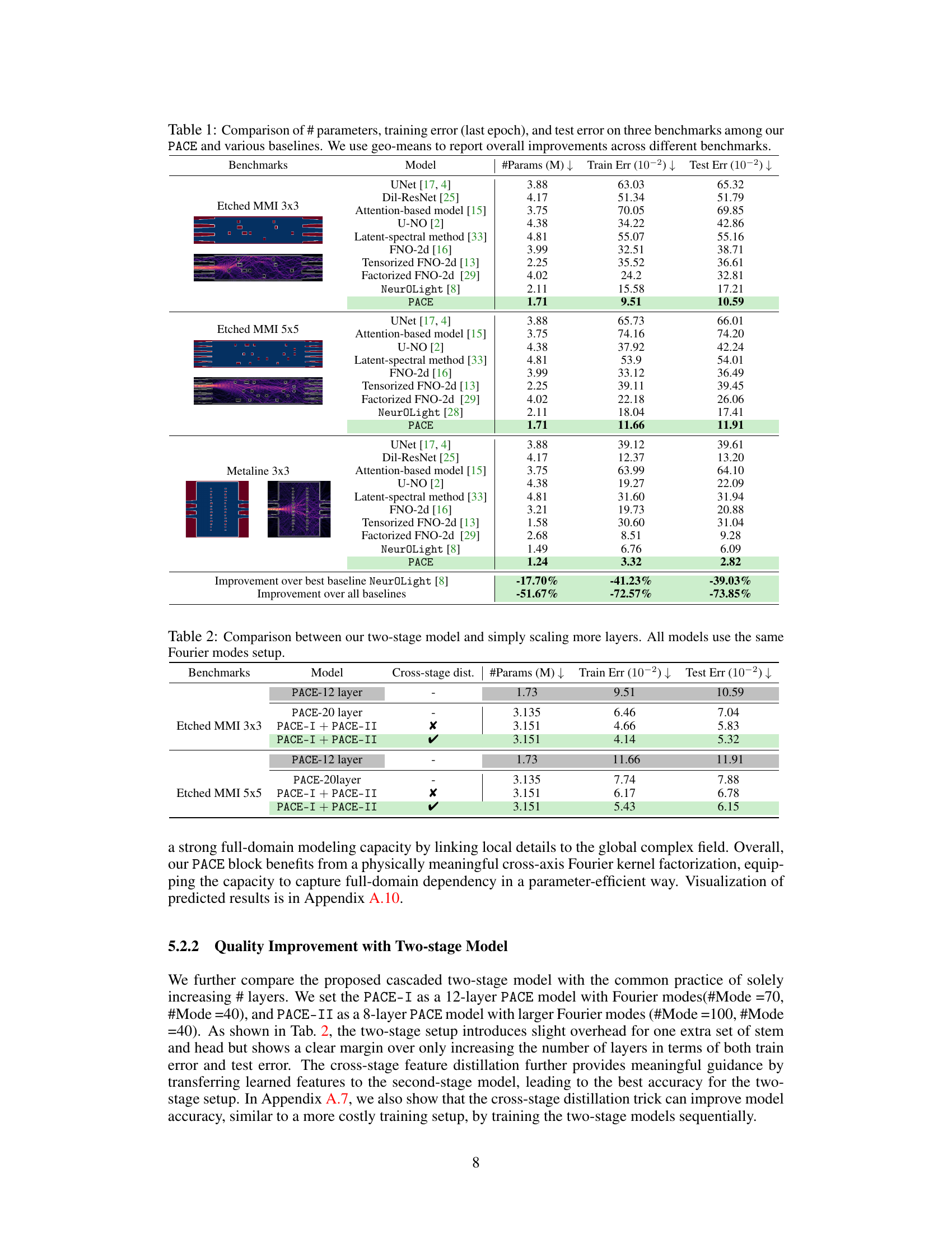
This table compares the performance of a single 12-layer PACE model, a single 20-layer PACE model, and a two-stage PACE model (with and without cross-stage feature distillation) on two benchmarks: Etched MMI 3x3 and Etched MMI 5x5. The results show that the two-stage model outperforms the single-stage models in terms of test error and that cross-stage feature distillation further improves performance.

This table presents the ablation study of the proposed PACE operator on the Metaline dataset. It shows the impact of removing the self-weighted path, the projection unit, and using TFNO instead of the PACE operator on the model’s performance, measured by the number of parameters, training error, and test error. The results highlight the importance of each component in achieving high accuracy.
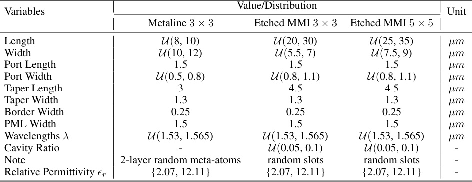
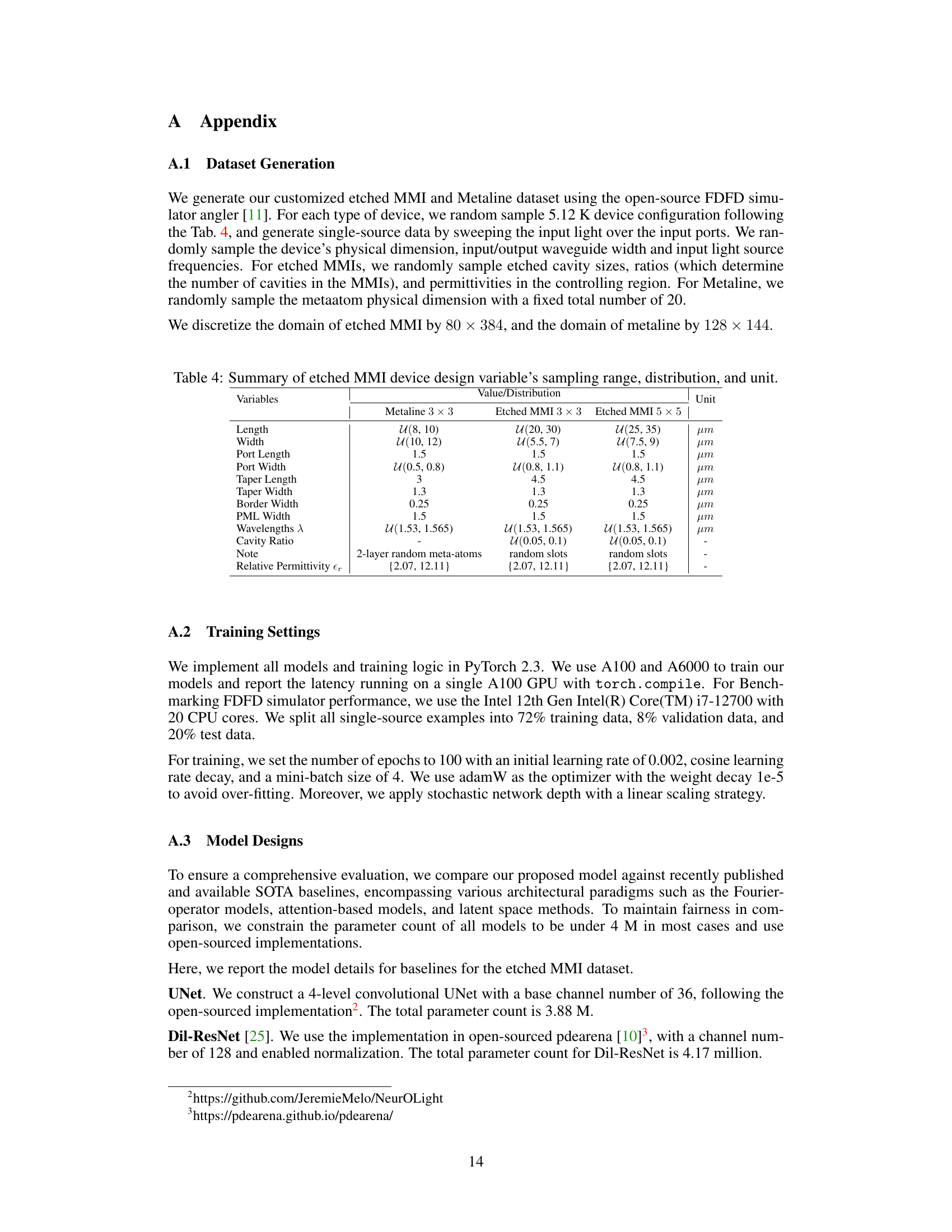
This table details the ranges and distributions of various design parameters used in the generation of the etched MMI datasets. It lists the variables (Length, Width, Port Length, Port Width, Taper Length, Taper Width, Border Width, PML Width, Wavelengths λ, Cavity Ratio, Relative Permittivity εr), their units (µm or -), and the value/distribution used in generating both the 3x3 and 5x5 etched MMI device datasets, as well as the Metaline 3x3 device dataset. Understanding this table is key to replicating the dataset generation process and interpreting the results in the paper. The use of uniform distributions and ranges is clearly indicated.

This table presents an ablation study on the impact of the number of groups (g) in the PACE operator on model performance. It shows that varying the number of groups affects both the number of parameters and the training and testing errors. The results suggest that a group size of 4 provides a good balance between model complexity (number of parameters) and accuracy (training and testing errors).

This table compares the performance of PACE and NeuroLight models with and without double skip connections and pre-normalization. It shows that adding both techniques improves the performance of both models, especially PACE. The table shows the number of parameters, training error, and test error for each model configuration.

This table compares the performance of the proposed two-stage PACE model against a single PACE model with increased layers. It shows the number of parameters, training error, and testing error for both models on two benchmark datasets (Etched MMI 3x3 and Etched MMI 5x5). The cross-stage distillation technique is also investigated to show its impact on the model’s performance. The results demonstrate the effectiveness of the two-stage approach, particularly when cross-stage distillation is utilized.
Full paper#
