↗ OpenReview ↗ NeurIPS Homepage ↗ Chat
TL;DR#
Bayesian inference for linear mixed-effects models (LMMs) often uses computationally expensive Markov Chain Monte Carlo (MCMC) methods, especially when dealing with many random effects. A common approach involves writing the model in a probabilistic programming language and sampling via HMC; however, model transformations can significantly affect the efficiency of this process. Marginalizing random effects is one such transformation that often proves beneficial but is difficult to implement.
This paper introduces a new algorithm that efficiently marginalizes random effects in LMMs. The key is to use a vectorized approach and fast linear algebra techniques to avoid expensive computations. The researchers demonstrate improvements in both speed and efficiency across a variety of models, particularly those with many variables and group-level effects, highlighting the broad applicability of this method. The findings suggest that marginalizing group-level effects should be a standard practice for Bayesian hierarchical modeling.
Key Takeaways#
Why does it matter?#
This paper is crucial for researchers working with linear mixed-effects models (LMMs). It offers a novel algorithm for efficient marginalization, a technique that significantly speeds up Bayesian inference, leading to faster and more accurate results. This is particularly important for large datasets common in many fields and opens new avenues for exploring more complex LMMs.
Visual Insights#
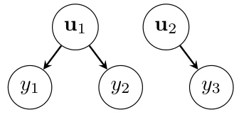
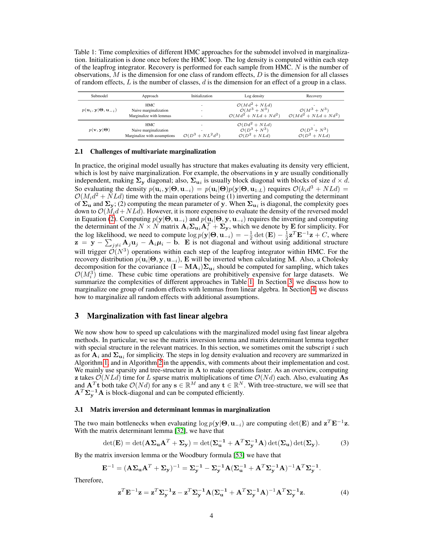
This figure is a graphical model showing the conditional independence structure of a linear mixed-effects model. The nodes represent variables, and the edges represent conditional dependencies. Θ represents the global variables (fixed effects and hyperparameters), u1 and u2 are random effects (e.g., for different subjects or groups), and y1, y2, and y3 are observations. The tree structure is crucial for efficient computations in the marginalization algorithm.

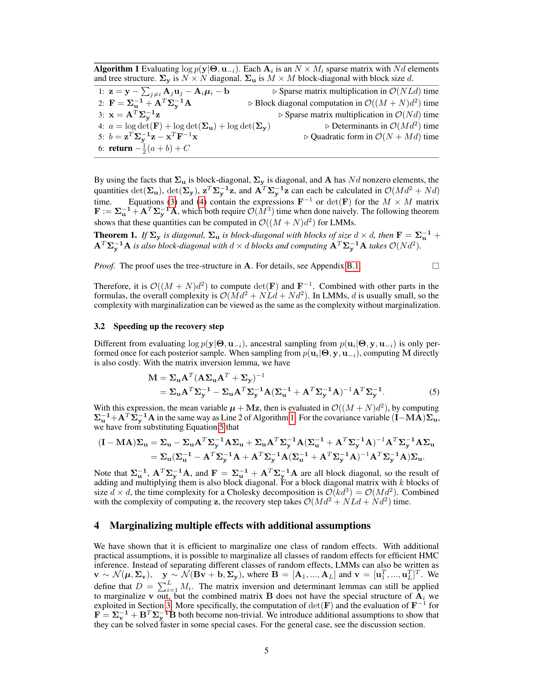
This table compares the time complexities of different Hamiltonian Monte Carlo (HMC) approaches used for marginalizing random effects in linear mixed-effects models (LMMs). It breaks down the computational cost into three phases: initialization (done once before the main HMC loop), log density computation (repeated in each step of the leapfrog integrator within the HMC algorithm), and recovery (performed for each sample generated by HMC). The complexities are expressed in terms of N (number of observations), M (dimension of one class of random effects), D (dimension of all classes of random effects), L (number of classes), and d (dimension of random effects per group). Three approaches are compared: standard HMC on the original model, naive marginalization, and marginalization with the proposed linear algebra optimizations.
In-depth insights#
Marginalized LMMs#
Marginalized Linear Mixed-Effects Models (LMMs) offer a significant advantage in Bayesian inference by analytically integrating out random effects. This simplifies the model, reducing the dimensionality of the parameter space for Hamiltonian Monte Carlo (HMC) sampling and thus improving its efficiency. The resulting marginalized likelihood, while potentially computationally complex, can be efficiently evaluated using fast linear algebra techniques, avoiding cubic-time operations associated with naive approaches. The benefits extend beyond computational speed, as marginalization also addresses pathologies in LMMs like the funnel shape caused by correlations between variance parameters and random effects, leading to improved sampling performance. The technique’s applicability, shown to be beneficial across various models, is particularly noteworthy for computationally intensive applications in cognitive sciences where hierarchical structures are prevalent, showcasing the practical impact of this methodological advancement.
HMC Efficiency#
Hamiltonian Monte Carlo (HMC) is a powerful Markov Chain Monte Carlo (MCMC) algorithm for Bayesian inference, but its efficiency can be significantly impacted by the model’s structure and parameterization. Marginalizing out nuisance parameters in linear mixed-effects models (LMMs) is shown to be a highly effective strategy to enhance HMC performance. A naive approach to marginalization can introduce cubic time complexities, but the authors present an optimized method using fast linear algebra techniques, reducing the time to linear complexity. This improvement dramatically speeds up the HMC sampler, particularly beneficial for LMMs with many random effects, as observed in experiments involving cognitive science datasets. The key to this efficiency gain lies in exploiting the structure of the linear model and utilizing efficient linear algebra operations such as the matrix inversion lemma, thereby mitigating the computational burden associated with high-dimensional integration. The empirical results demonstrate substantial improvements in both Effective Sample Size (ESS) and runtime, underlining the practical advantages of the proposed marginalization method for improving the efficiency of HMC in Bayesian inference for LMMs.
Linear Algebra#
The effective application of linear algebra is crucial for efficiently handling the high-dimensional computations inherent in Bayesian inference for linear mixed-effects models (LMMs). The paper leverages fast linear algebra techniques to overcome the cubic time complexity associated with naive marginalization of random effects, reducing it to linear time. This improvement is achieved primarily through the clever application of the matrix inversion lemma and matrix determinant lemma. These lemmas, combined with the exploitation of sparse and tree-structured matrices, enable efficient computation of key quantities within the Hamiltonian Monte Carlo (HMC) algorithm. The resulting linear time complexity ensures scalability for large datasets. Vectorization is employed to further enhance efficiency, highlighting a significant contribution of the paper. The use of these established linear algebra tools to solve a statistical problem illustrates a novel and potentially widely applicable approach for enhancing HMC algorithms.
Cognitive Models#
Cognitive models, in the context of a research paper, would likely explore how humans process information. A key aspect would be the computational modeling of cognitive processes, potentially using Bayesian methods to represent uncertainty and build hierarchical models. The paper might delve into specific cognitive functions such as attention, memory, or language, examining how these are implemented in computational frameworks. Another focus could be the evaluation and validation of cognitive models, possibly comparing them to empirical data from behavioral experiments or neuroimaging studies. This would likely involve the development of specific model architectures and algorithms, with detailed analysis of efficiency and scalability. The work might emphasize the use of probabilistic programming languages, which offer advantages in representing uncertainty and complex relationships within the model.
Future Work#
The paper’s discussion of future work highlights several promising avenues. Extending marginalization techniques beyond normal likelihoods is crucial for broader applicability, particularly to models with probit regressions or other non-normal distributions. This requires investigation into simulation-based methods or variational approaches. Efficiently marginalizing multiple random effects in general models poses a significant challenge, suggesting the need for algorithms that can effectively handle high-dimensional covariance matrices and large datasets, potentially using stochastic estimators and techniques like pseudo-marginalization. Finally, seamless integration of marginalization into probabilistic programming languages would automate the process, making the technique more accessible to users. This would involve developing algorithms to automatically recognize and apply marginalization within existing PPLs, potentially extending their functionality and improving the efficiency of Bayesian inference in a wide range of complex models.
More visual insights#
More on figures

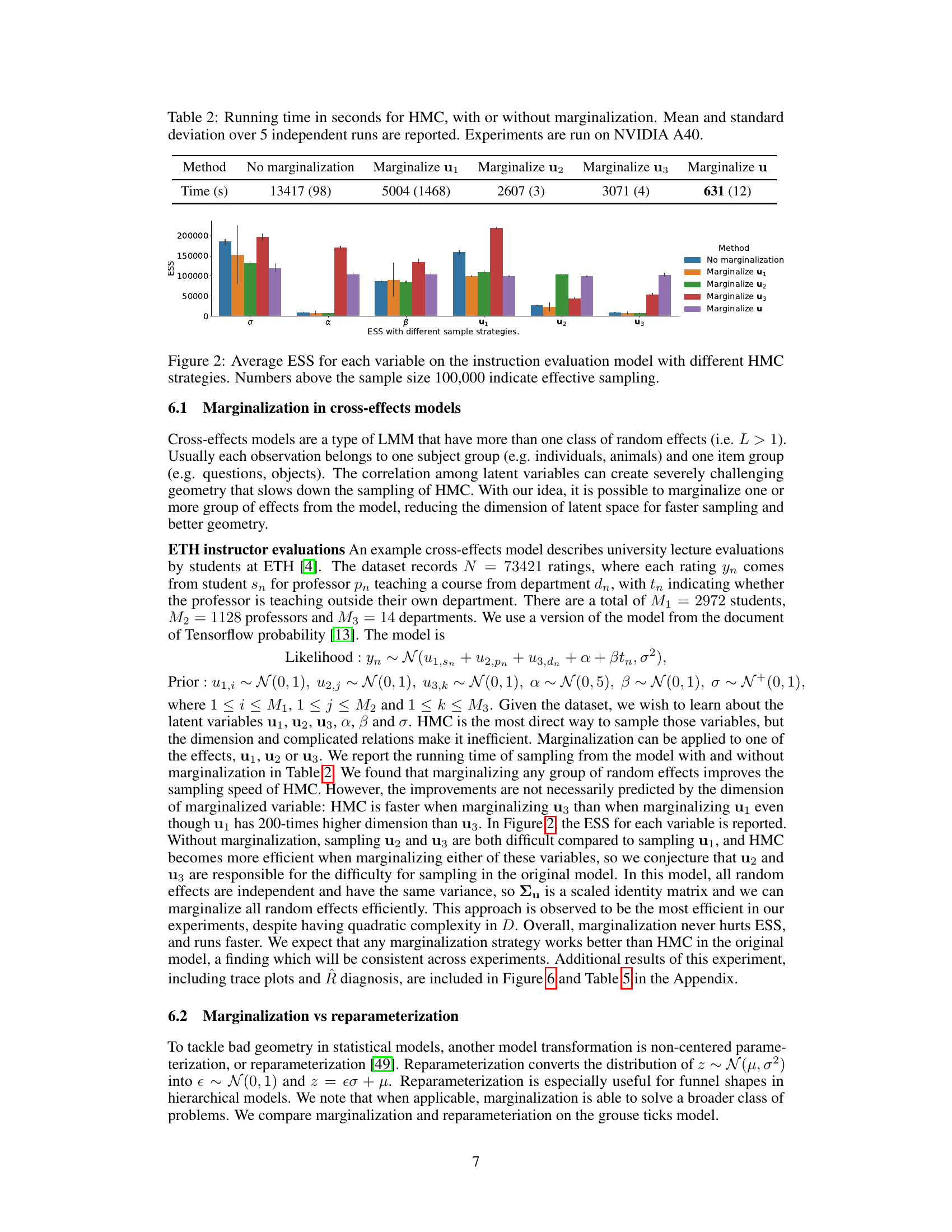
This figure compares the Effective Sample Size (ESS) per variable for different Hamiltonian Monte Carlo (HMC) sampling strategies applied to the ETH instructor evaluation model. The strategies include no marginalization and marginalizing different groups of random effects (u1, u2, u3, or all u’s). The higher the ESS, the more efficient the sampling for that variable. Numbers above the bars indicate that effective sample size is above the 100,000 samples collected.

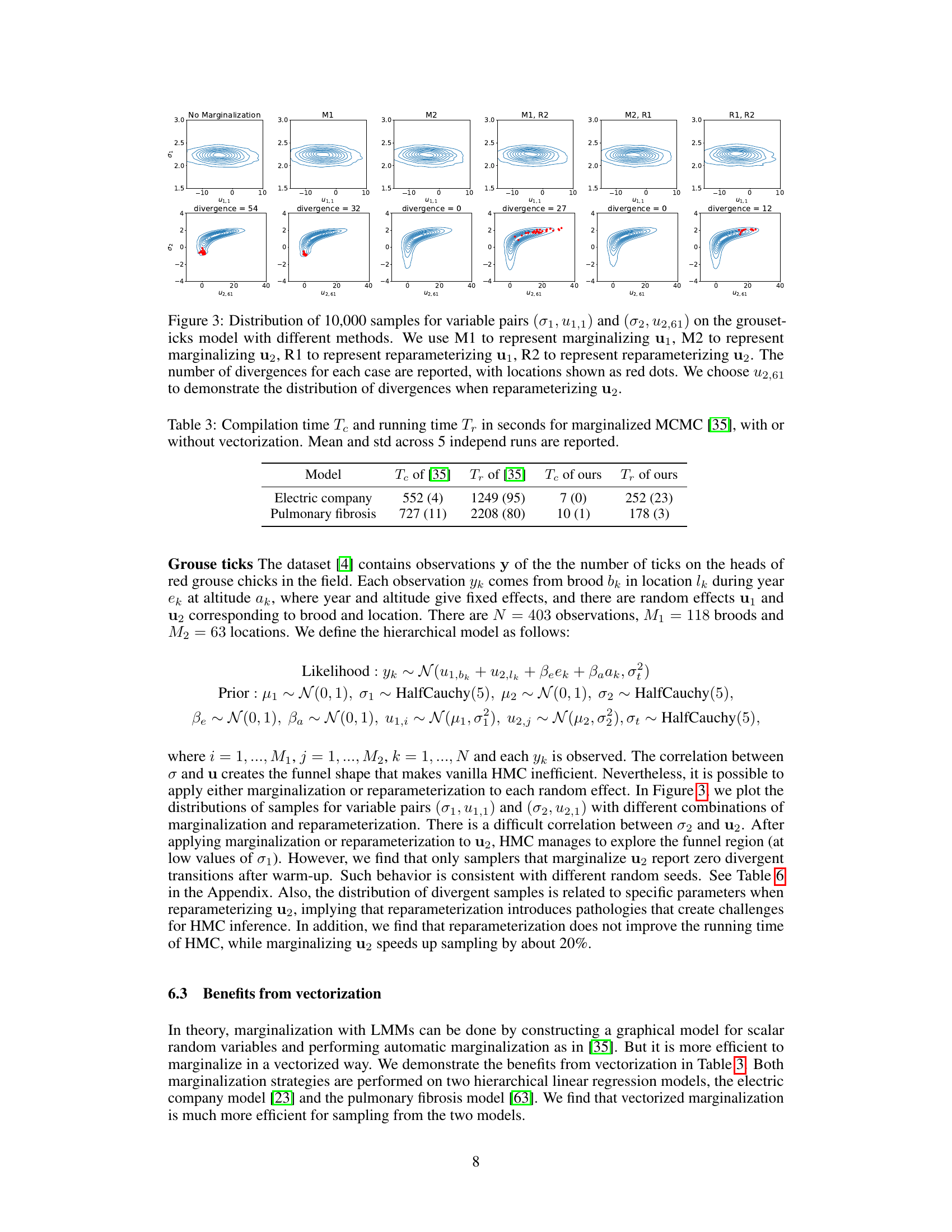
This figure compares the performance of marginalization and reparameterization on the grouse ticks model by visualizing the distributions of 10,000 samples for variable pairs (σ1, u1,1) and (σ2, u2,61). Different methods are compared: no marginalization, marginalizing u1, marginalizing u2, marginalizing u1 and reparameterizing u2, marginalizing u2 and reparameterizing u1, and reparameterizing u1 and u2. Red dots represent divergences. The figure shows that marginalization generally leads to better sampling behavior with fewer divergences, especially when marginalizing u2.
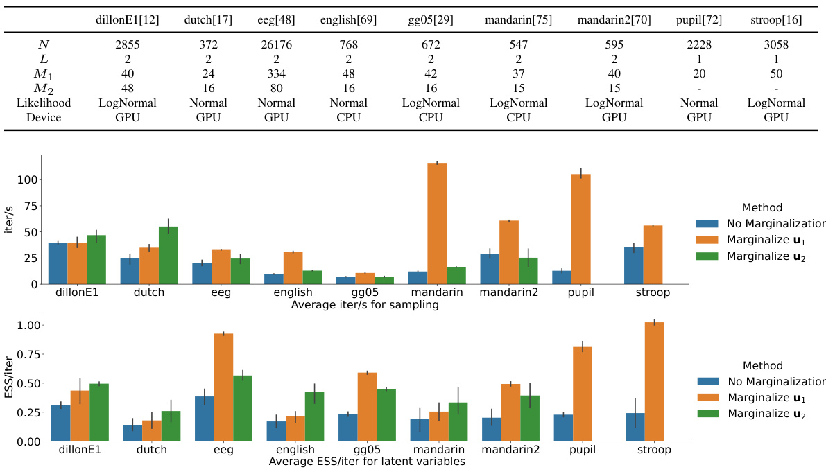
This figure presents the experimental results of applying the proposed marginalization technique to nine different cognitive science datasets. The results are compared against the standard Hamiltonian Monte Carlo (HMC) approach without marginalization. The figure displays two key metrics: iterations per second (iter/s) representing sampling speed, and effective sample size per iteration (ESS/iter) indicating sample efficiency. Error bars are included to show variability across the five runs with different random seeds for each dataset and method. The results demonstrate that marginalization generally leads to faster sampling (higher iter/s) and more efficient sampling (higher ESS/iter) in most cases.
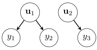
This figure is a graphical representation of a linear mixed-effects model (LMM) with a tree structure. The nodes represent variables, with Θ representing global variables (like hyperparameters), u1 and u2 representing random effects, and y1, y2, and y3 representing observations. The arrows indicate conditional dependencies: the observations depend on the random effects, and the random effects depend on the global variables. This tree structure is crucial for the efficiency of the marginalization algorithm described in the paper, as it allows for computationally efficient matrix operations.
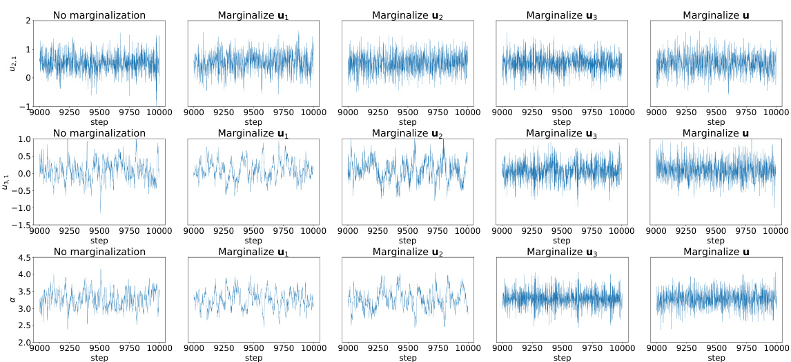
This figure shows the trace plots of three variables (α2,1, α3,1, and σ) from the ETH instructor evaluation model after a 1000 sampling steps warmup period. The trace plots illustrate the convergence behavior of the Markov chain Monte Carlo (MCMC) sampling process for these parameters under different marginalization strategies. The purpose is to visually assess the mixing properties and stability of the MCMC sampler when marginalizing different sets of random effects (u1, u2, u3, or all of them).

This figure compares the performance of marginalization and reparameterization on the grouse ticks model. It shows the distribution of 10,000 samples for two pairs of variables, (σ1, u1,1) and (σ2, u2,61), under different sampling strategies: marginalizing u1 (M1), marginalizing u2 (M2), reparameterizing u1 (R1), and reparameterizing u2 (R2). The number of divergences (HMC sampling failures) is also reported for each case, highlighted with red dots. The plots illustrate how marginalization effectively addresses the problematic correlations that hinder efficient sampling in the original model, while reparameterization is less successful in this regard.

This figure compares the performance of marginalization and reparameterization in handling the funnel shape pathology in the grouse ticks model. It shows the distributions of samples for two pairs of variables, highlighting the impact of each method on sampling efficiency and the occurrence of divergences (indicated by red dots). The results demonstrate that marginalization effectively addresses the funnel problem and reduces divergences, whereas reparameterization may still suffer from some pathologies, leading to a higher number of divergences.

This figure compares the performance of marginalization and reparameterization on a specific model (grouse ticks model) by visualizing the distribution of samples for selected variable pairs (σ1, u1,1) and (σ2, u2,61). The different methods used are marginalization of u1 (M1), marginalization of u2 (M2), reparameterization of u1 (R1), and reparameterization of u2 (R2). Red dots indicate divergences. The plots reveal that marginalization is better at avoiding divergences than reparameterization in this model.
More on tables

This table compares the time complexities of different Hamiltonian Monte Carlo (HMC) approaches for marginalizing random effects in linear mixed-effects models (LMMs). It breaks down the computational cost of initialization, log density evaluation, and recovery steps for various marginalization methods, highlighting the impact of model structure and algorithm choices on efficiency. The complexities are expressed in terms of N (number of observations), M (dimension of one class of random effects), D (dimension of all classes), L (number of classes), and d (dimension of an effect in a group).

This table presents the average running time (in seconds) of the Hamiltonian Monte Carlo (HMC) algorithm for different marginalization strategies on the ETH instructor evaluation model. It compares the original model (No marginalization) with four other variations where either u1, u2, u3, or all random effects (u) are marginalized. The results are averages across five independent runs, with standard deviations included in parentheses.

This table compares the compilation time (Te) and running time (Tr) of the marginalized MCMC method proposed in the paper [35] with the authors’ vectorized approach. The comparison is done for two models: Electric company and Pulmonary fibrosis. The results show significant improvements in both compilation and running times using the proposed vectorized approach.

This table compares the time complexities of different Hamiltonian Monte Carlo (HMC) approaches for performing marginalization in linear mixed-effects models. It breaks down the complexities for initialization, computing the log density (within each step of the leapfrog integrator), and the recovery step (for each sample from HMC). The complexities are expressed in terms of N (number of observations), M (dimension of one class of random effects), D (dimension of all classes of random effects), L (number of classes of random effects), and d (dimension of an effect of a group in a class).

This table compares the time complexities of different Hamiltonian Monte Carlo (HMC) approaches for marginalizing random effects in linear mixed-effects models (LMMs). It breaks down the computational cost of initialization, computing the log density (within each leapfrog step of the HMC algorithm), and recovering marginalized variables for each sample. The complexities are expressed in terms of N (number of observations), M (dimension of one class of random effects), D (dimension of all random effects), L (number of classes), and d (dimension of an effect in a group).

This table compares the computational complexities of different Hamiltonian Monte Carlo (HMC) approaches used for marginalizing random effects in linear mixed-effects models. It breaks down the complexities for initialization, computing the log density (which is done repeatedly within the HMC algorithm), and the recovery step (which is done once per sample). The complexities are expressed in terms of N (number of observations), M (dimension of one class of random effects), D (dimension of all classes), L (number of classes), and d (dimension of one effect).

This table shows the number of divergences encountered during Hamiltonian Monte Carlo (HMC) sampling for the grouse ticks model under various conditions. The conditions involve different combinations of marginalizing (M1, M2) and reparameterizing (R1, R2) two different random effects (u1 and u2) in the model. The results are averaged over five independent runs with different random seeds, illustrating the impact of these transformations on HMC’s sampling performance in terms of divergences, which are a measure of problematic steps taken by the sampler.
Full paper#

