A Primal-Dual-Assisted Penalty Approach to Bilevel Optimization with Coupled Constraints

uZi7H5Ac0X

Liuyuan Jiang et el.

TL;DR
#

Bilevel optimization (BLO) is increasingly important in machine learning but existing methods struggle with coupled constraints across the upper and lower levels. These coupled constraints frequently appear in complex real-world applications such as hyperparameter tuning and network design, significantly limiting the applicability of existing BLO algorithms. This paper addresses these limitations by focusing on BLO problems with coupled constraints, which is an under-explored and challenging scenario.

This research introduces BLOCC, a fully first-order algorithm, that efficiently solves bilevel optimization problems with coupled constraints. Unlike previous approaches, BLOCC avoids computationally expensive joint projections, enabling faster computation and improved scalability. The algorithm’s effectiveness is demonstrated through theoretical analysis and real-world applications. Rigorous convergence guarantees are established, making BLOCC a reliable tool for various machine learning applications.

Key Takeaways
#

Why does it matter?
#

This paper is crucial for researchers working on bilevel optimization, particularly those dealing with complex real-world problems involving coupled constraints. It offers a novel, efficient algorithm and rigorous theoretical backing, opening avenues for tackling previously intractable problems in machine learning and beyond. The improved scalability and convergence properties of the proposed method are particularly significant for large-scale applications.

Visual Insights
#

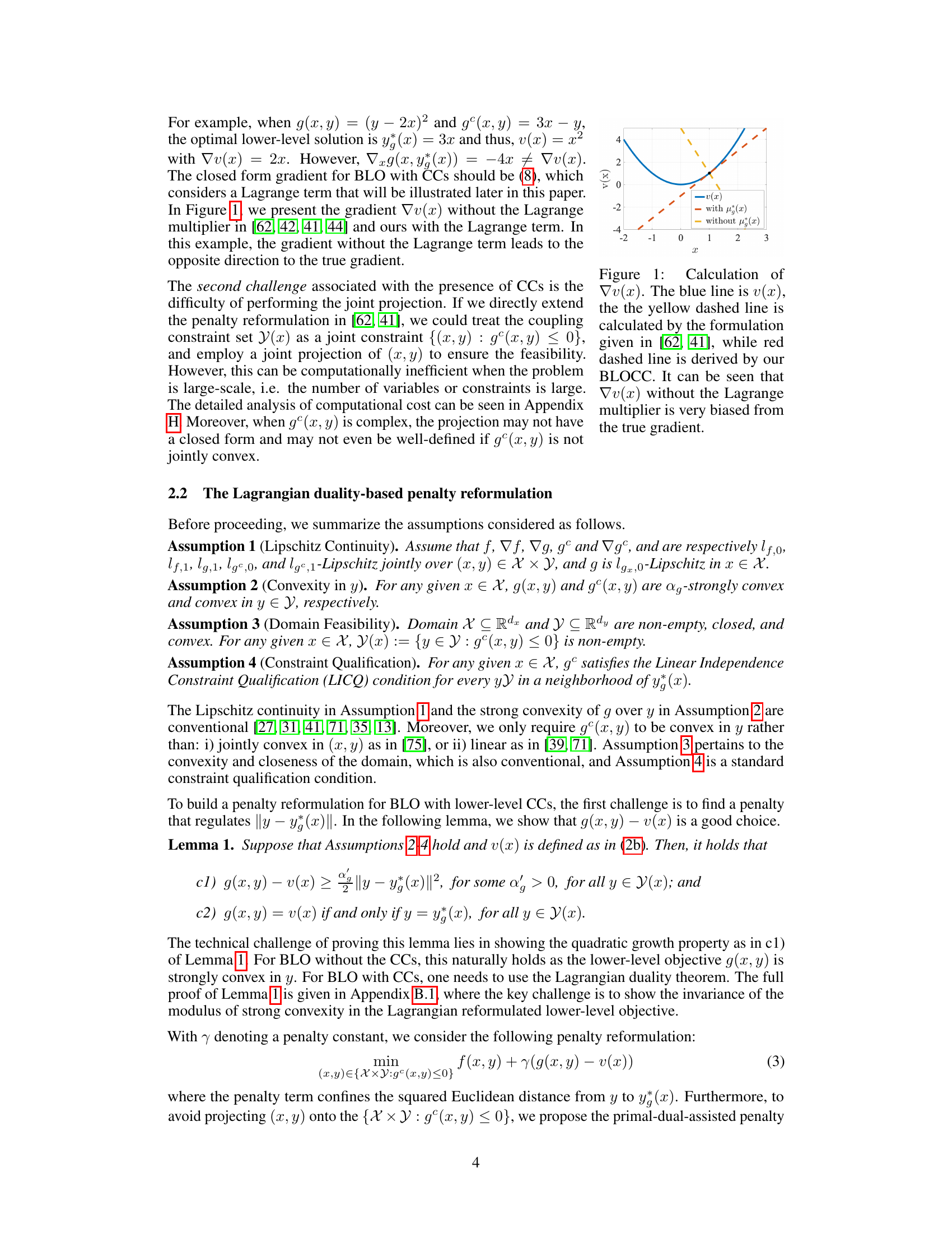
This figure compares three different methods for calculating the gradient of the value function v(x) in a bilevel optimization problem with coupled constraints. The blue line shows the true gradient. The yellow dashed line represents a previously proposed method that doesn’t account for coupled constraints, resulting in a significantly inaccurate gradient. The red dashed line shows the gradient calculated by the proposed BLOCC algorithm, which is much closer to the true gradient. This highlights the importance of correctly handling coupled constraints when calculating the gradient.

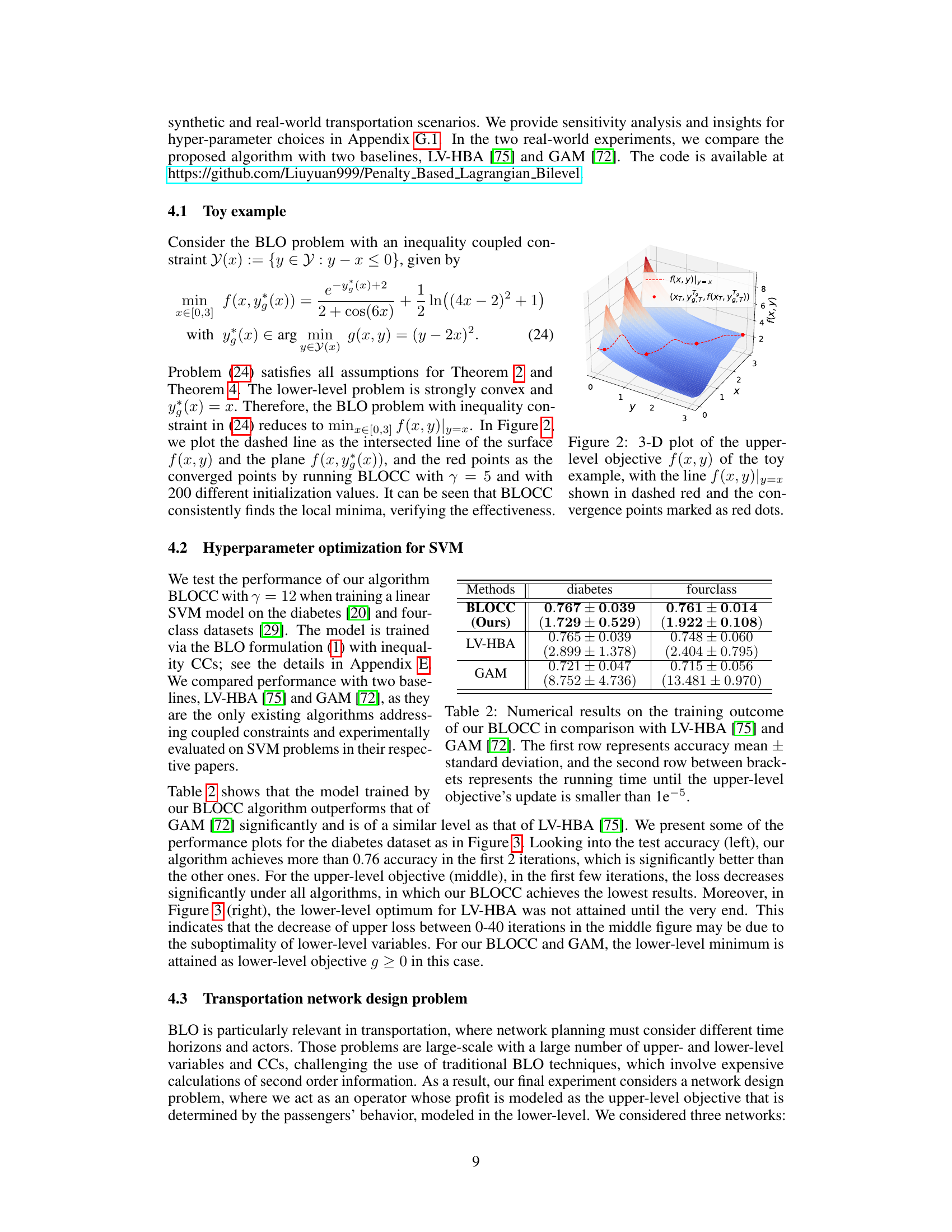
This table compares the proposed BLOCC algorithm with four other state-of-the-art algorithms for solving bilevel optimization problems with coupled constraints. It highlights key differences in the types of constraints handled, whether the algorithm is first-order, and the achieved convergence complexity (both upper and lower level). The table shows that BLOCC offers improvements in terms of constraint generality and convergence rate.

In-depth insights
#

BLOCC Algorithm
#

The BLOCC algorithm, a novel approach to bilevel optimization with coupled constraints, tackles the challenge of optimizing problems where upper and lower levels are intertwined. Its core innovation lies in a primal-dual-assisted penalty reformulation, cleverly sidestepping the computationally expensive joint projection step typically required for handling coupled constraints in such problems. By introducing a penalty term and Lagrangian term in its reformulation, it decouples the upper and lower-level variables and thus improves the computational efficiency. This reformulation’s smoothness and favorable properties facilitate the use of gradient-based methods. The algorithm’s rigorous convergence theory is established, demonstrating finite-time convergence guarantees under specified assumptions. Importantly, BLOCC’s efficiency is validated through empirical results on real-world applications such as SVM hyperparameter tuning and transportation network planning, showcasing its effectiveness for large-scale problems. The algorithm’s adaptability and robustness is particularly significant in addressing the challenges posed by coupled constraints, making it a valuable contribution to the field of bilevel optimization.

Penalty Reformulation
#

Penalty reformulation is a crucial technique in bilevel optimization, aiming to transform a challenging bilevel problem into a more tractable single-level one. This typically involves introducing penalty terms to the objective function, penalizing violations of constraints or discrepancies between the upper and lower levels. A well-designed penalty function is key; it needs to balance the approximation accuracy with computational cost. Strong convexity and smoothness assumptions are often crucial for theoretical guarantees of convergence and efficient algorithms. The choice of penalty parameter also plays a significant role; too small a parameter might not sufficiently penalize violations, while too large a parameter might lead to numerical instability. The effectiveness of penalty reformulation depends heavily on the problem structure and the properties of the objective functions and constraints, highlighting the importance of careful design and analysis.

Convergence Analysis
#

A rigorous convergence analysis is crucial for establishing the reliability and efficiency of any algorithm. In the context of bilevel optimization, convergence analysis becomes particularly challenging due to the nested structure and coupled constraints. A well-structured analysis should start by clearly stating the assumptions made about the problem’s properties (e.g., convexity, smoothness, Lipschitz continuity). The analysis should then demonstrate how these assumptions are used to prove the algorithm’s convergence properties. Key aspects to analyze include the rate of convergence (linear, sublinear, etc.), and the factors affecting this rate (e.g., problem parameters, step sizes, and the presence of constraints). The analysis must also address the impact of any approximations or simplifications made during the algorithm’s design. The analysis should ideally include proofs for the convergence theorems. Furthermore, the analysis should discuss the practical implications of the convergence results, highlighting how the findings relate to the algorithm’s computational cost and overall effectiveness. A comprehensive analysis would cover both theoretical convergence guarantees and empirical performance evaluation, showing a strong correlation between the two. Finally, sensitivity analysis of convergence with respect to algorithm parameters is important to assess the robustness of the proposed approach.

SVM & Networks
#

The combination of Support Vector Machines (SVMs) and network analysis presents a powerful paradigm for tackling complex data-driven problems. SVMs excel at classification and regression tasks, particularly in high-dimensional spaces, offering a robust framework for pattern recognition. When integrated with network data, SVMs can leverage the rich relational information embedded within networks, allowing for more nuanced modeling that goes beyond isolated nodes or features. This synergy is particularly valuable in applications such as social network analysis, where predicting user behavior or detecting communities often requires understanding the contextual influence of connections. Similarly, biological networks benefit from SVM analysis, as protein-protein interaction data can be harnessed to predict protein function or disease progression. However, challenges remain. The computational complexity of SVMs can be significant, especially for large networks with dense connections. Feature engineering for network data also presents a challenge, as effective representation methods must capture both local and global network properties. Ultimately, the success of applying SVMs to network analysis hinges on careful consideration of these challenges, requiring a balance between modeling accuracy and computational efficiency. Research into scalable algorithms and efficient feature representation techniques for network data will be crucial for advancing this field.

Future Work
#

The paper’s “Future Work” section could explore several promising avenues. Extending BLOCC to handle more complex constraint structures beyond coupled inequalities is crucial. This might involve non-convex constraints, equality constraints, or even stochastic constraints. Improving the scalability of BLOCC further is also important. While the paper demonstrates progress, tackling truly massive datasets and high-dimensional problems remains a challenge. Investigating alternative optimization methods or developing sophisticated approximation techniques could enhance scalability. A deeper theoretical analysis of BLOCC’s convergence properties under weaker assumptions would solidify its foundations. The current assumptions, while reasonable, could be relaxed to broaden applicability. Finally, the authors could focus on developing more practical applications of BLOCC in real-world scenarios beyond the presented examples. This would require careful consideration of data acquisition, preprocessing, model selection, and interpretation of results. Focusing on specific, high-impact applications could significantly enhance the paper’s impact.

More visual insights
#

More on figures

The figure compares three different methods to calculate the gradient of the value function v(x). The blue line shows the actual value function v(x). The yellow dashed line represents the gradient calculated using a previous method from the literature (references [62, 41]), which does not consider the Lagrange multiplier. The red dashed line shows the gradient calculated using the BLOCC method proposed in the paper, which incorporates the Lagrange multiplier. The figure demonstrates that the previous method significantly underestimates the gradient, highlighting the importance of including the Lagrange multiplier in the calculation.

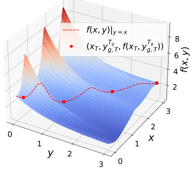
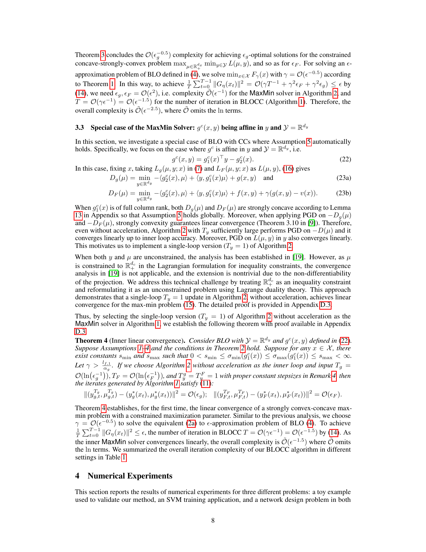
This figure shows a 3D plot of the upper-level objective function f(x, y) for a toy example problem. The dashed red line represents the values of f(x, y) when y is constrained to equal x (y = x). The red dots represent the points where the BLOCC algorithm converged for 200 different initializations. The plot visually demonstrates the algorithm’s ability to consistently find the local minima.

The figure shows the results of applying the BLOCC algorithm to train a linear SVM model on the diabetes dataset. Three metrics are plotted against the number of iterations: test accuracy, upper-level loss (validation loss), and lower-level loss. The plots show mean values (bold lines) and standard deviations (shaded regions) across 50 different random train-validation-test splits of the data. The figure helps to illustrate the performance of the BLOCC algorithm in terms of convergence speed and accuracy in a real-world machine learning application.

The figure shows the test accuracy, validation loss (upper level), and lower-level objective for the diabetes dataset. Three algorithms, BLOCC, LV-HBA, and GAM, are compared in terms of their performance over running time and iteration count. The plots show mean values and shaded regions representing standard deviations across multiple runs.

This figure illustrates an example of a transportation network design problem. It shows the input topology (a), demand matrix (b), constructed network (c), and passengers served by the constructed network (d). The input topology shows the stations and links with associated travel times. The demand matrix represents the travel demand between each origin-destination pair. The constructed network shows the links selected by the optimization algorithm, with the thickness of the links representing their capacity. Finally, the passengers served matrix shows the number of passengers using the constructed network for each origin-destination pair.

The figure shows the performance of BLOCC and LV-HBA algorithms for a 3-node network design problem. The upper-level objective function f(xt, yt) is plotted against the running time. Solid lines represent the mean of f(xt, yg,t), while dashed lines represent the mean of f(xt, yft), with shaded regions indicating standard deviations. Three different values of the penalty parameter γ are compared (γ = 2, 3, and 4), along with the LV-HBA algorithm (orange line). The plot visualizes the convergence speed and the impact of γ on the objective function value.

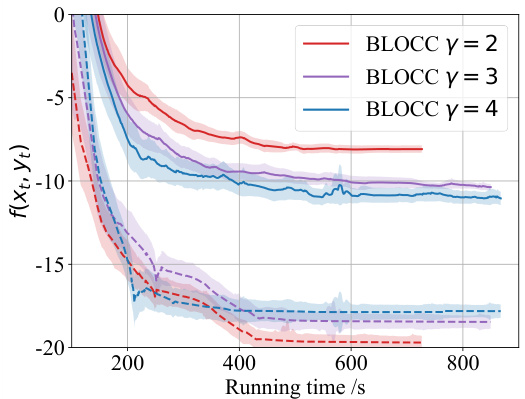
The figure shows the performance of the BLOCC algorithm and LV-HBA algorithm on a 3-node network design problem. The x-axis represents the running time, while the y-axis represents the upper-level objective function value. Solid lines represent the mean of f(xt, ygt), while dashed lines represent the mean of f(xt, yFt). The shaded regions represent standard deviations. Different colors represent different values of the penalty parameter γ, and the orange line represents the result from the LV-HBA algorithm.

This figure shows the convergence of the upper-level objective function f(xt, yt) for a 3-node network design problem over time. The solid lines represent the mean value of the objective function using yg,t (obtained from the lower-level optimization with Tg iterations), while the dashed lines represent the mean using yFt (obtained from the lower-level optimization with TF iterations). The shaded regions represent the standard deviation. Three different values of the penalty parameter γ are shown (red, purple, and blue). The orange line shows results obtained using the LV-HBA algorithm, a baseline algorithm for comparison.

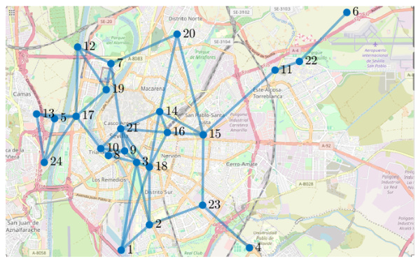
This figure shows the topology of the Seville metro network used in the transportation network design problem in Section 4.3. It displays the 24 potential station locations (nodes) and the 88 links (edges) connecting them, based on proximity and travel time constraints. The map shows the geographical layout of the stations within the city of Seville.

TL;DR#

Key Takeaways#

Why does it matter?#

Visual Insights#

In-depth insights#

BLOCC Algorithm#

Penalty Reformulation#

Convergence Analysis#

SVM & Networks#

Future Work#

More visual insights#

Full paper#