TL;DR#
Continual data streams are ubiquitous in today’s applications, but preserving privacy in such scenarios poses a significant challenge. Traditional differential privacy mechanisms often assume uniform sensitivity across all data points which is unrealistic. The paper focuses on continual counting, a fundamental primitive for many stream processing tasks and introduces the issue of privacy with expiration, where the privacy loss granted to a data item diminishes as time passes. Existing methods either provide weak privacy guarantees or are computationally expensive.
This work proposes a novel algorithm that addresses the issues of privacy in continual counting under gradual privacy expiration. The algorithm boasts an additive error of O(log(T)/ε), matching a lower bound proved by the authors, and it provides optimal error for a wide range of privacy expiration functions. The improved accuracy is achieved while maintaining scalability, demonstrated through both theoretical analysis and empirical evaluations that shows its effectiveness against natural baseline algorithms.
Key Takeaways#
Why does it matter?#
This paper is crucial for researchers in differential privacy because it addresses the significant challenge of continual data streams where data sensitivity decreases over time. It bridges the gap between theory and practice by offering a novel algorithm that achieves optimal accuracy with gradual privacy expiration, opening doors for more practical and efficient privacy-preserving systems in dynamic environments. This is especially timely given increasing concerns about data privacy in modern applications.
Visual Insights#

🔼 This figure illustrates how the noise is added to the prefix sum in Algorithms 2 and 3. It shows two streams, x and y, differing only in the third position. The nodes represent dyadic intervals. Filled nodes indicate intervals where noise is shifted to achieve the same output for both streams up to time step 6. Bold nodes represent the intervals contributing to the noise for the fourth prefix sum calculation.
read the caption
Figure 1: An example of the noise structure for Algorithm 2 and Algorithm 3 for B = 0 on two neighbouring streams x and y differing in position 3. The nodes correspond to the dyadic intervals. The filled nodes mark the intervals I for which the noise Z1 is shifted by one between x and y to get the same outputs for T = 6. The fat nodes mark the intervals I corresponding to the Z1 which are used in the computation of the fourth prefix sum s4.

🔼 This table lists the privacy parameters (ε, εcur, εpast) used in the plots shown in Figures 3 and 4. For each plot, these parameters were chosen to achieve a mean-squared error (MSE) of 1000 over the stream length T. The parameters vary based on the algorithm (Algorithm 3 or the baseline), the value of λ (for Algorithm 3), and the window size W (for the baseline).
read the caption
Table 1: Table over the privacy parameters used in each of the plots.
In-depth insights#
Gradual Privacy#
The concept of ‘Gradual Privacy’ in the context of continual observation addresses the evolving sensitivity of data over time. Traditional differential privacy treats all data points equally, regardless of their age. However, in many real-world scenarios (e.g., location tracking, website visits), recent data is significantly more sensitive than older data. Gradual privacy models this by allowing the privacy parameter (ε) to decrease as data ages. This means a stronger privacy guarantee is provided for newer data while older data has a progressively weaker guarantee. The key challenge lies in designing algorithms that offer this gradual decay of privacy while maintaining sufficient accuracy. This necessitates careful trade-offs: stronger privacy for recent data comes at the cost of increased error (noise), potentially affecting the utility of older data. The optimal trade-off depends heavily on the specific application and the chosen privacy expiration function. Research in this area focuses on developing new algorithms and establishing theoretical bounds on accuracy and privacy loss for different functions, seeking optimal solutions for a broad range of sensitivity changes. The ultimate goal is to create a versatile framework that dynamically adapts to the ever-changing sensitivity of streaming data, providing privacy guarantees that are both meaningful and practical.
Continual Counting#
Continual counting, in the context of differential privacy, presents a unique challenge: continuously releasing a statistic (e.g., a count) from a data stream while preserving privacy. The core difficulty lies in balancing the need for accurate updates with the inherent privacy loss associated with each release of information. Traditional approaches often face a trade-off between accuracy and privacy, especially when dealing with long streams, as the cumulative privacy loss can become significant. This paper tackles the problem by introducing the concept of gradual privacy expiration, where the privacy guarantee for older data points gradually decreases over time. This approach allows for more frequent updates and higher accuracy without excessively compromising overall privacy. The authors present innovative algorithms that achieve optimal accuracy under these conditions, providing both theoretical bounds and empirical validation. Their algorithm significantly improves upon existing methods in terms of accuracy, while maintaining a controlled and carefully analyzed privacy loss. The introduction of gradual privacy expiration represents a significant advancement in the field, as it provides a more practical and realistic model for many real-world applications where data sensitivity diminishes with time.
Privacy Bounds#
Analyzing privacy bounds in a differential privacy context involves a careful examination of the trade-offs between privacy protection and utility. Tight bounds are crucial, as they provide precise guarantees on the level of privacy preservation achieved by a mechanism. Loose bounds, on the other hand, might offer weaker assurances and could lead to overestimation of privacy. The paper likely investigates different types of privacy bounds, such as those for specific privacy models (e.g., pure differential privacy vs. approximate differential privacy), accounting for the impact of parameters like epsilon (ε) and the privacy loss function (g(d)). It explores how the type of privacy bound affects the overall accuracy of the algorithm. A key aspect is the relationship between the privacy bounds and the algorithmic error. The research probably aims to demonstrate that even with gradual privacy expiration, achieving optimal error bounds is feasible for certain classes of privacy functions. Therefore, analyzing these aspects of privacy bounds leads to a deeper understanding of the algorithm’s behavior and its suitability for specific applications where privacy concerns are paramount.
Algorithm Analysis#
A thorough algorithm analysis should dissect the paper’s proposed algorithms for continual counting with gradual privacy expiration. This involves examining runtime complexity, ideally differentiating between amortized and worst-case scenarios, and analyzing space complexity, noting any dependence on stream length or other parameters. Crucially, the analysis must rigorously prove privacy guarantees, demonstrating adherence to the defined ε-differential privacy with expiration function g(d). This requires a detailed examination of the noise-adding mechanisms and their impact on the privacy loss at various time points. Accuracy analysis is equally critical, establishing bounds on additive error and ideally providing probabilistic guarantees on the error’s magnitude. The analysis should be mathematically precise, explicitly stating assumptions and presenting clear, verifiable proofs. Comparisons to existing continual counting algorithms are essential, highlighting the advantages and disadvantages of the novel approach in terms of accuracy, privacy, and resource usage, ideally with a quantitative comparison of error bounds under similar privacy parameters.
Future Work#
The continual counting problem with gradual privacy expiration, as explored in this paper, presents exciting avenues for future research. Extending the framework to approximate differential privacy is a crucial next step, as this would broaden the applicability of the findings and potentially improve privacy-utility trade-offs. Investigating slower-growing expiration functions and algorithms for other problems in continual observation (e.g., maintaining histograms, frequency-based statistics) would further enrich this line of work. The substantial gap between batch and continual release models in problems like max-sum and counting distinct elements presents a strong motivation to explore whether the gradual privacy expiration model can yield better trade-offs. Finally, the direct applicability of these algorithms to privacy-preserving federated learning warrants further investigation, especially regarding optimization in the stochastic gradient descent setting.
More visual insights#
More on figures
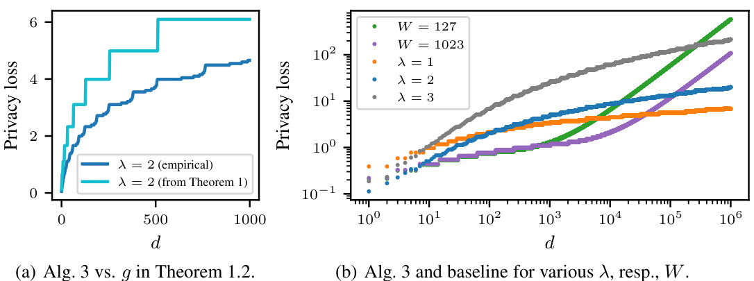
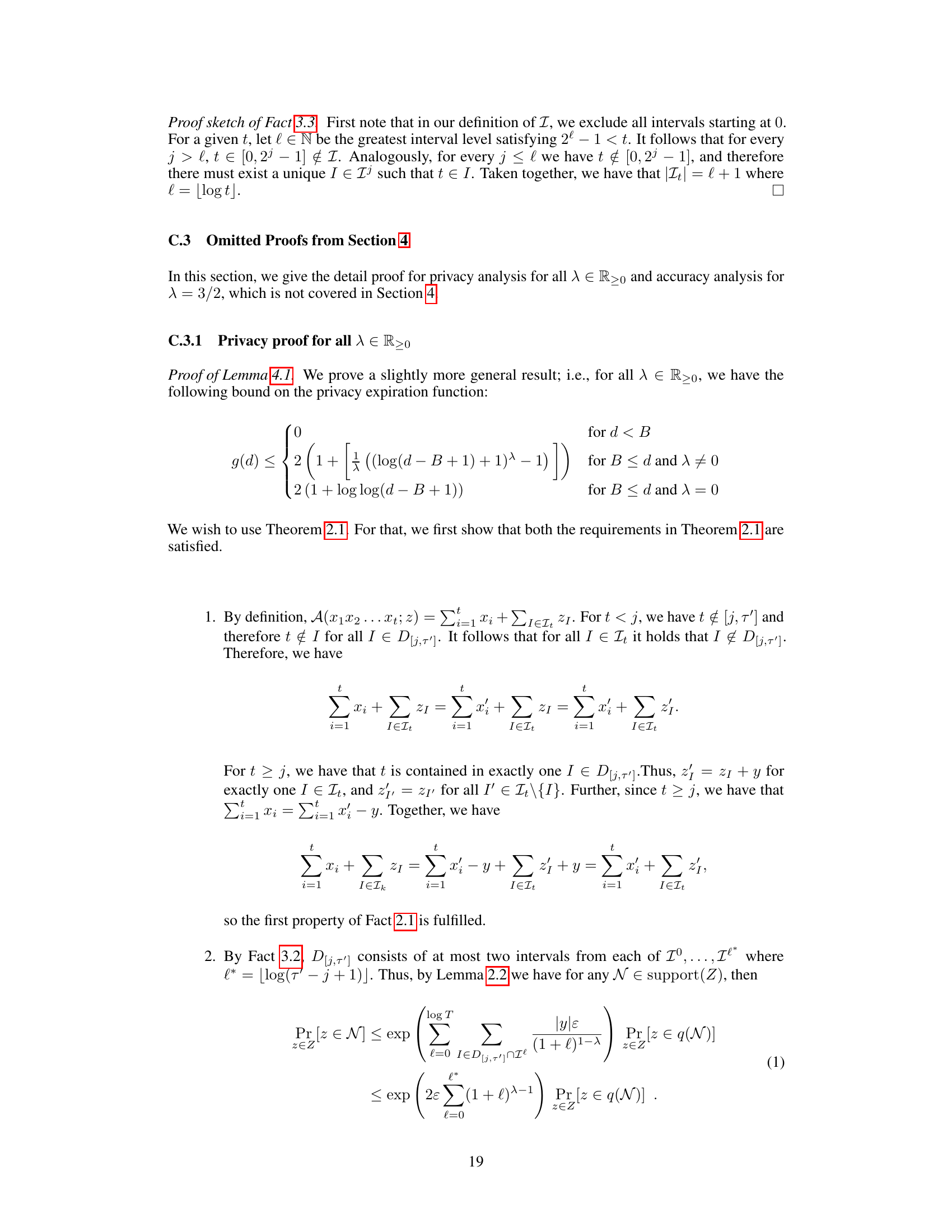
🔼 This figure displays two plots visualizing privacy loss. Plot (a) compares the empirically observed privacy loss of Algorithm 3 (for λ = 2) to the theoretical privacy loss predicted by Theorem 1.2 (also for λ = 2). Plot (b) contrasts the privacy loss of Algorithm 3 (for various values of λ) with that of a baseline algorithm (for different window sizes W). The plots show the relationship between privacy loss and the elapsed time (d) since a data item was streamed. The baseline algorithm represents a more conventional continual counting approach.
read the caption
Figure 2: Plots on the privacy loss for our Algorithm 3 and a baseline algorithm.

🔼 The plots show the privacy loss for Algorithm 3 and a baseline algorithm for different parameters. Subfigure (a) compares the empirical privacy loss of Algorithm 3 to the theoretical privacy loss given by Theorem 1.2, showing a close match and polylogarithmic growth. Subfigure (b) compares Algorithm 3 to the baseline algorithm for various parameters (λ and W respectively), highlighting that Algorithm 3 achieves a significantly smaller empirical privacy loss for large values of d than the baseline.
read the caption
Figure 2: Plots on the privacy loss for our Algorithm 3 and a baseline algorithm.

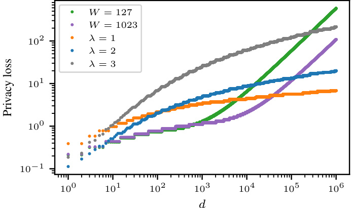
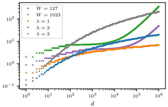
🔼 This figure presents empirical results about privacy loss in continual counting with gradual privacy expiration. Subfigure (a) compares the empirically computed privacy loss with the theoretical bound from Theorem 1.2. Subfigure (b) illustrates how Algorithm 3’s privacy loss changes based on parameter λ. Subfigure (c) shows the baseline algorithm’s privacy loss with varied parameter W. The results demonstrate that Algorithm 3 offers a slower-growing privacy loss compared to the baseline, especially for larger values of the respective parameters.
read the caption
Figure 3: Worst-case privacy loss computed empirically for a data item streamed d steps earlier. (a) Alg. 3 vs. g in Theorem 1.2. (b) Algorithm 3 for multiple λ. (c) Baseline for multiple W.
🔼 This figure compares the privacy loss of Algorithm 3 (continual counting with gradual privacy expiration) to a baseline algorithm. Figure 2(a) shows how well the theoretical privacy loss function (from Theorem 1.2) approximates the empirically observed privacy loss for Algorithm 3, demonstrating a polylogarithmic growth in both. Figure 2(b) compares Algorithm 3 with various parameters (λ) to the baseline algorithm with different parameters (W), showing that Algorithm 3 achieves significantly smaller empirical privacy loss for large values of the elapsed time (d) than the baseline.
read the caption
Figure 2: Plots on the privacy loss for our Algorithm 3 and a baseline algorithm.

🔼 This figure shows three plots visualizing the empirically computed worst-case privacy loss for a data item that was streamed d steps earlier, for Algorithm 3 and a baseline algorithm. Plot (a) compares the empirically computed privacy loss with the theoretical privacy loss given by Theorem 1.2, showing a good match. Plot (b) demonstrates the impact of parameter λ on Algorithm 3’s privacy loss, showing that larger λ results in higher privacy loss for large d but lower loss for small d. Plot (c) illustrates the effect of parameter W (window size) on the baseline algorithm’s privacy loss, demonstrating that linear privacy expiration emerges for large enough d.
read the caption
Figure 3: Worst-case privacy loss computed empirically for a data item streamed d steps earlier. (a) Alg. 3 vs. g in Theorem 1.2. (b) Algorithm 3 for multiple λ. (c) Baseline for multiple W.
🔼 Figure 2(a) compares the empirical privacy loss of Algorithm 3 to the theoretical privacy loss given by Theorem 1.2. It shows that the theoretical bound is a good approximation of the empirical privacy loss. Figure 2(b) compares the privacy loss of Algorithm 3 with different parameters (λ) to the privacy loss of a baseline algorithm. For large enough d, Algorithm 3 has a smaller privacy loss than the baseline.
read the caption
Figure 2: Plots on the privacy loss for our Algorithm 3 and a baseline algorithm.
Full paper#
