TL;DR#
Visual Place Recognition (VPR) is critical for mobile robots, enabling key functions like localization and mapping. Traditional VPR often faces challenges such as perspective changes, seasonal variations, and occlusions. Existing fine-tuning methods for Visual Foundation Models (VFMs) often overlook the importance of probing in adapting descriptors for better image representation.
This paper introduces EMVP, a new parameter-efficient fine-tuning pipeline for VPR. EMVP utilizes a novel Centroid-Free Probing (CFP) stage and a Dynamic Power Normalization (DPN) module. CFP effectively uses second-order features from VFMs, while DPN adaptively controls the preservation of task-specific information. Experimental results demonstrate EMVP’s superiority over existing methods, achieving state-of-the-art results on multiple benchmark datasets with significantly reduced trainable parameters.
Key Takeaways#
Why does it matter?#
This paper is crucial for researchers in visual place recognition (VPR) because it introduces a novel parameter-efficient fine-tuning (PEFT) pipeline, EMVP, that significantly improves VPR accuracy and efficiency. EMVP leverages Visual Foundation Models (VFMs) and introduces Centroid-Free Probing (CFP) and Dynamic Power Normalization (DPN) to enhance the adaptation of VFMs to VPR tasks. This addresses the challenges of traditional VPR methods that often involve training a model from scratch on environment-specific data. The enhanced efficiency and improved accuracy open up new research directions for resource-constrained VPR applications.
Visual Insights#
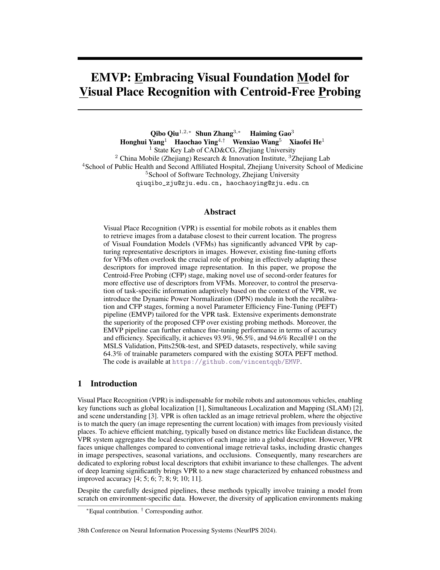
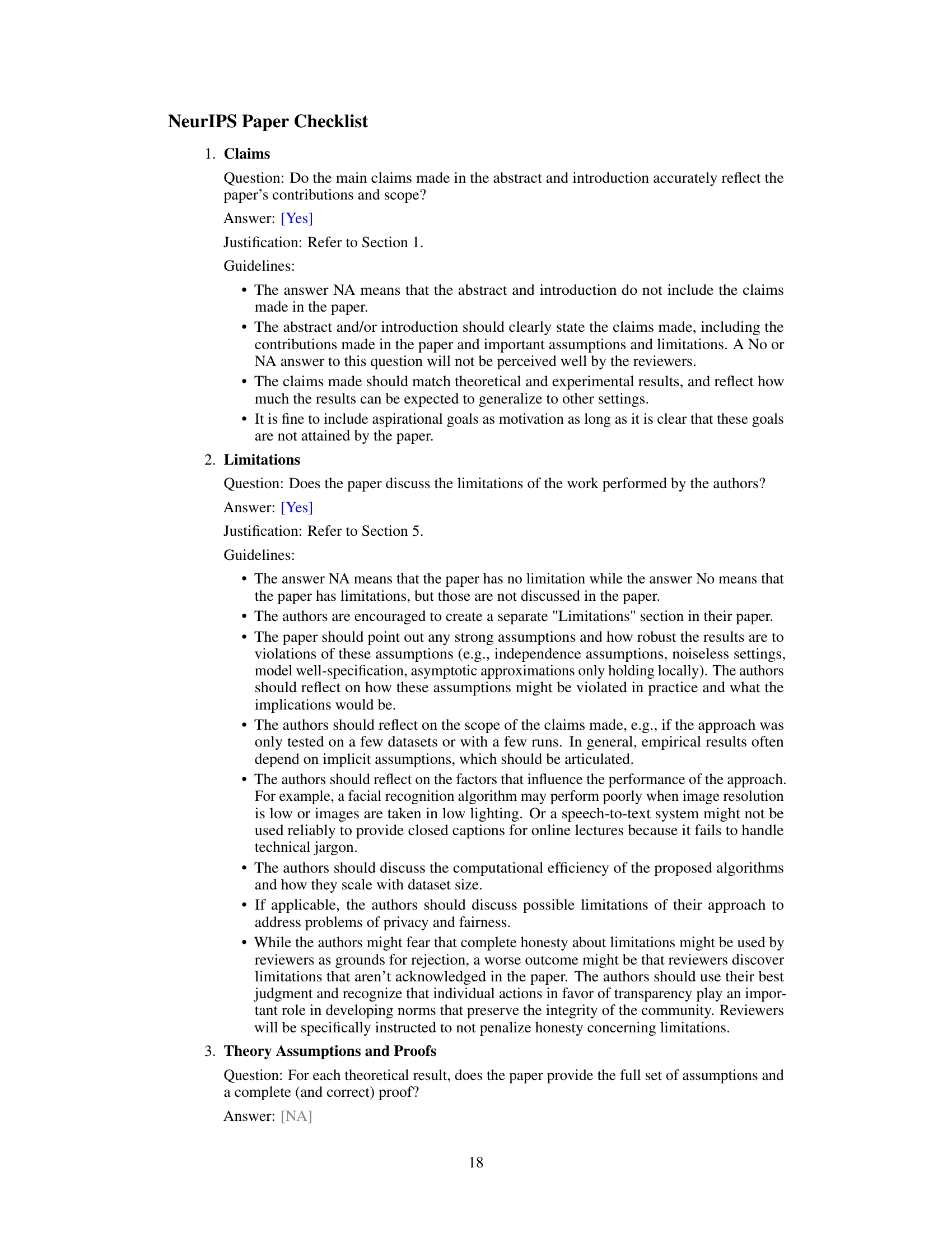
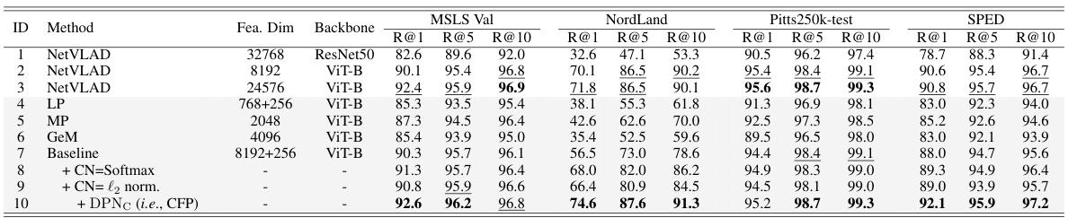
🔼 This figure compares four different probing methods used for visual place recognition. Linear Probing (LP) uses simple averaging or max-pooling of features. GeM pooling is a generalization of LP. NetVLAD uses more sophisticated aggregation that requires initialization of centroids. The authors’ proposed Centroid-Free Probing (CFP) simplifies NetVLAD while improving performance and interpretability by removing the centroid initialization step.
read the caption
Figure 1: Comparison of different probing methods. (a) The most popular Linear Probing (LP) in classification fine-tuning. (b) Generalized-Mean (GeM) pooling adapted by SelaVPR [13], which can be seen as a generalized form of first-order feature. (c) The NetVLAD operation simplified by SALAD [12]. (d) The proposed Centroid-Free Probing (CFP) which provides a theoretical and empirical justification for this simplification, fixing interpretability and performance issues that were present otherwise.
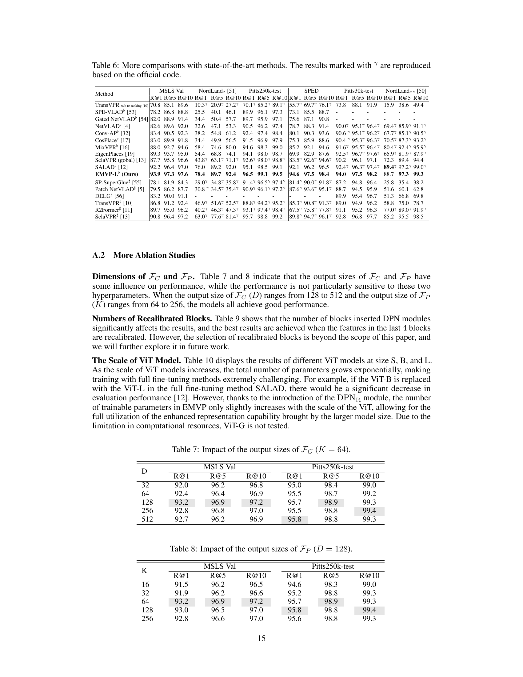
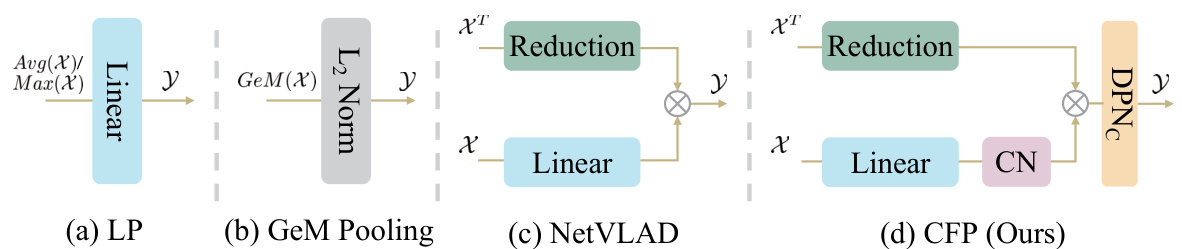
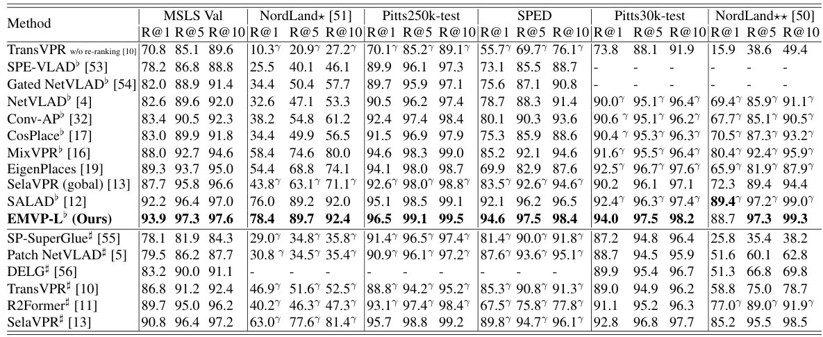
🔼 This table compares the proposed EMVP model’s performance on various visual place recognition datasets against other state-of-the-art methods. It highlights the recall rate (R@1, R@5, R@10) achieved by each method on the MSLS Validation, Nordland, Pitts250k-test, and SPED datasets. The table also indicates whether a method was trained on the GSV-Cities dataset, noting that methods trained on this high-quality dataset generally perform better.
read the caption
Table 1: Comparison with state-of-the-art methods. ♭ denotes models trained on the GSV-Cities dataset. Due to the high quality of annotations in GSV-Cities, results from models marked with ♭ generally outperform those from their corresponding papers. In contrast, results from models without ♭ are reported in their respective papers.
In-depth insights#
Centroid-Free Probing#
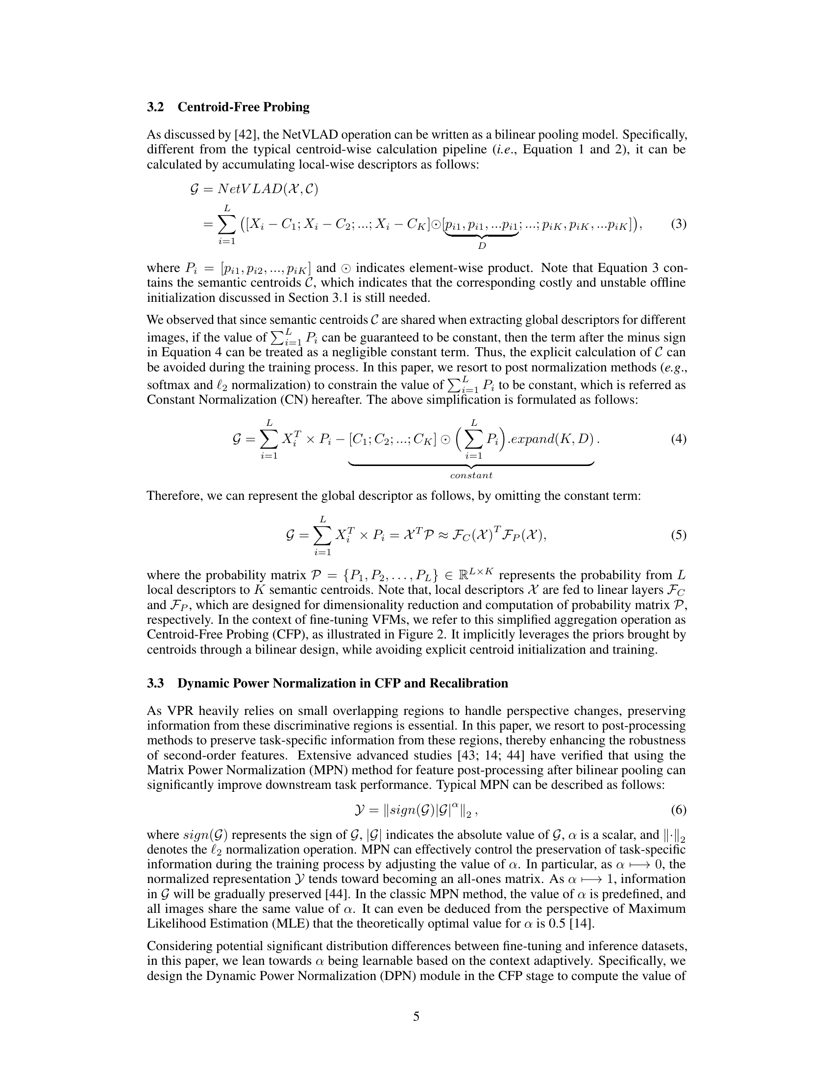
The concept of “Centroid-Free Probing” presents a novel approach to visual place recognition (VPR), specifically addressing limitations in existing methods. Traditional techniques often rely on NetVLAD, which necessitates the computationally expensive and potentially unstable initialization of semantic centroids. Centroid-Free Probing elegantly circumvents this by avoiding explicit centroid calculation, leveraging a constant normalization technique to ensure consistent aggregation of local descriptors. This simplification improves efficiency and mitigates the risk of introducing inductive bias from poorly initialized centroids. The method’s effectiveness is further enhanced by incorporating Dynamic Power Normalization (DPN) to adaptively control the preservation of task-specific information during the probing stage. This dynamic control is crucial for VPR, as it enables the system to focus on discriminative features, such as background elements often vital for place recognition, even when dealing with significant changes in perspective. Overall, Centroid-Free Probing offers a more efficient and robust alternative to traditional methods, providing valuable advancements in VPR.
Dynamic Power Norm#
The concept of “Dynamic Power Normalization” suggests an adaptive mechanism for controlling feature normalization, rather than using a static approach. This is particularly beneficial in scenarios where the importance of features might vary across different contexts or data points. The dynamic aspect is crucial, allowing the model to adjust its focus on specific features based on input characteristics. For example, in visual place recognition, the system might emphasize background details when there are drastic changes in viewpoint, while foreground object features hold more weight in other conditions. This adaptive normalization enhances robustness, enabling the model to better handle variability and noise inherent in the data. The technique likely involves learnable parameters that dynamically adjust the normalization strength based on input features, possibly using an additional network layer or module. This introduces non-linearity, improving the model’s ability to represent complex relationships. A well-designed dynamic normalization scheme would be computationally efficient, otherwise hindering performance.
VFM Fine-Tuning#
Visual Foundation Models (VFMs) offer a powerful new paradigm for visual place recognition (VPR), but effectively adapting their pretrained representations for this specific task remains a challenge. Fine-tuning VFMs for VPR often involves carefully balancing the need for task-specific adaptation with preserving the generalizability of the pretrained model. Strategies like adapter modules or prompt tuning offer parameter-efficient approaches, but may not fully exploit the rich representational capacity of the VFM. A key area of research involves exploring more sophisticated probing mechanisms that effectively aggregate local features into a robust global representation, potentially leveraging second-order statistics for improved discriminative power. Controlling the preservation of task-specific information is also crucial, especially for VPR which must address variations in viewpoint, lighting, and season. Methods such as dynamic normalization could help address this by adaptively focusing on task-relevant features. Ultimately, the success of VFM fine-tuning in VPR will depend on a nuanced combination of efficient adaptation techniques and strategies for preserving or enhancing task-specific information.
Ablation Study#
An ablation study systematically removes components of a model to determine their individual contributions. In the context of a visual place recognition model, this might involve removing or disabling specific modules (e.g., centroid-free probing, dynamic power normalization) to observe the impact on performance metrics like Recall@1. By comparing the full model’s performance to versions with components removed, researchers can isolate the effects of individual parts and assess their importance. This helps demonstrate the efficacy of the proposed design choices, clarifying which features are crucial for the model’s overall success and potentially suggesting areas for future improvement or simplification. The ablation study also supports the validity of design decisions and strengthens the paper’s claims by providing empirical evidence for the contributions of each component.
Future Directions#
Future research directions stemming from this work could explore several promising avenues. Extending the Centroid-Free Probing (CFP) method to other visual tasks beyond visual place recognition (VPR) is a key area. The inherent flexibility of CFP, focusing on second-order features, might prove beneficial in other applications needing robust global feature aggregation. Improving the Dynamic Power Normalization (DPN) module’s adaptability is also crucial. Investigating alternative strategies or more sophisticated learning mechanisms for dynamically adjusting the power normalization could enhance its effectiveness and reduce sensitivity to various image conditions. A thorough comparative study across different Visual Foundation Models (VFMs) would be insightful. The current research relies on DINOv2; comparing performance with other VFMs like CLIP or MAE may reveal valuable insights about the model’s generalizability and efficiency, potentially leading to improved fine-tuning strategies. Finally, the impact of combining EMVP with other VPR techniques, such as re-ranking methods, deserves further investigation. This integration may lead to enhanced overall accuracy and robustness, resulting in a more comprehensive VPR system.
More visual insights#
More on figures
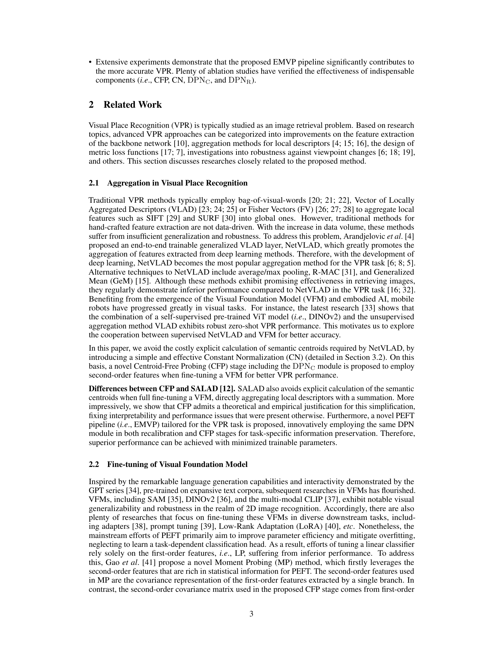
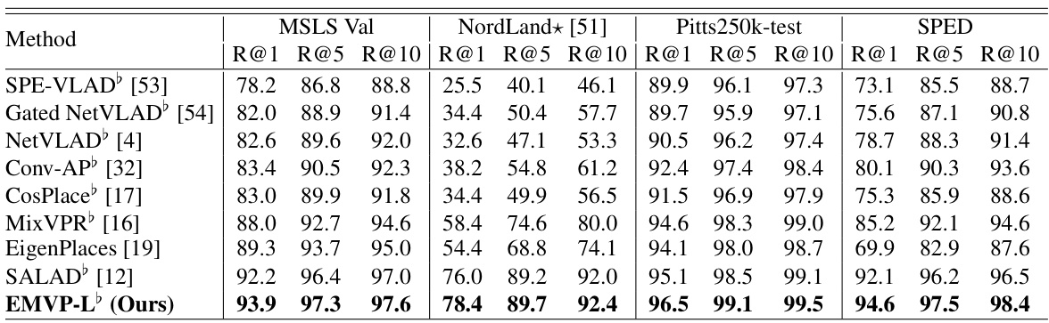
🔼 This figure illustrates the overall architecture of EMVP, a parameter-efficient fine-tuning pipeline for visual place recognition. It consists of two main stages: recalibration and centroid-free probing (CFP). The recalibration stage utilizes a dynamic power normalization (DPN) module to enhance task-specific information preservation in the backbone network. The CFP stage employs a novel centroid-free probing method that leverages second-order features for improved representation. Both stages use DPN for adaptive control of task-specific information.
read the caption
Figure 2: Overall pipeline of the proposed EMVP, including recalibration and CFP stages. Feature matrices from the two branches (i.e., Fc and FP) are multiplied to obtain fine-grained features for the improved VPR performance. The Dynamic Power Normalization (DPN) layer can be inserted into both the recalibration and CFP stages to enhance the task-specific fine-tuning performance.
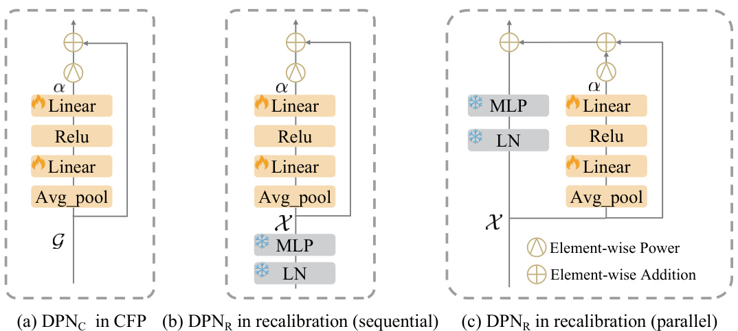
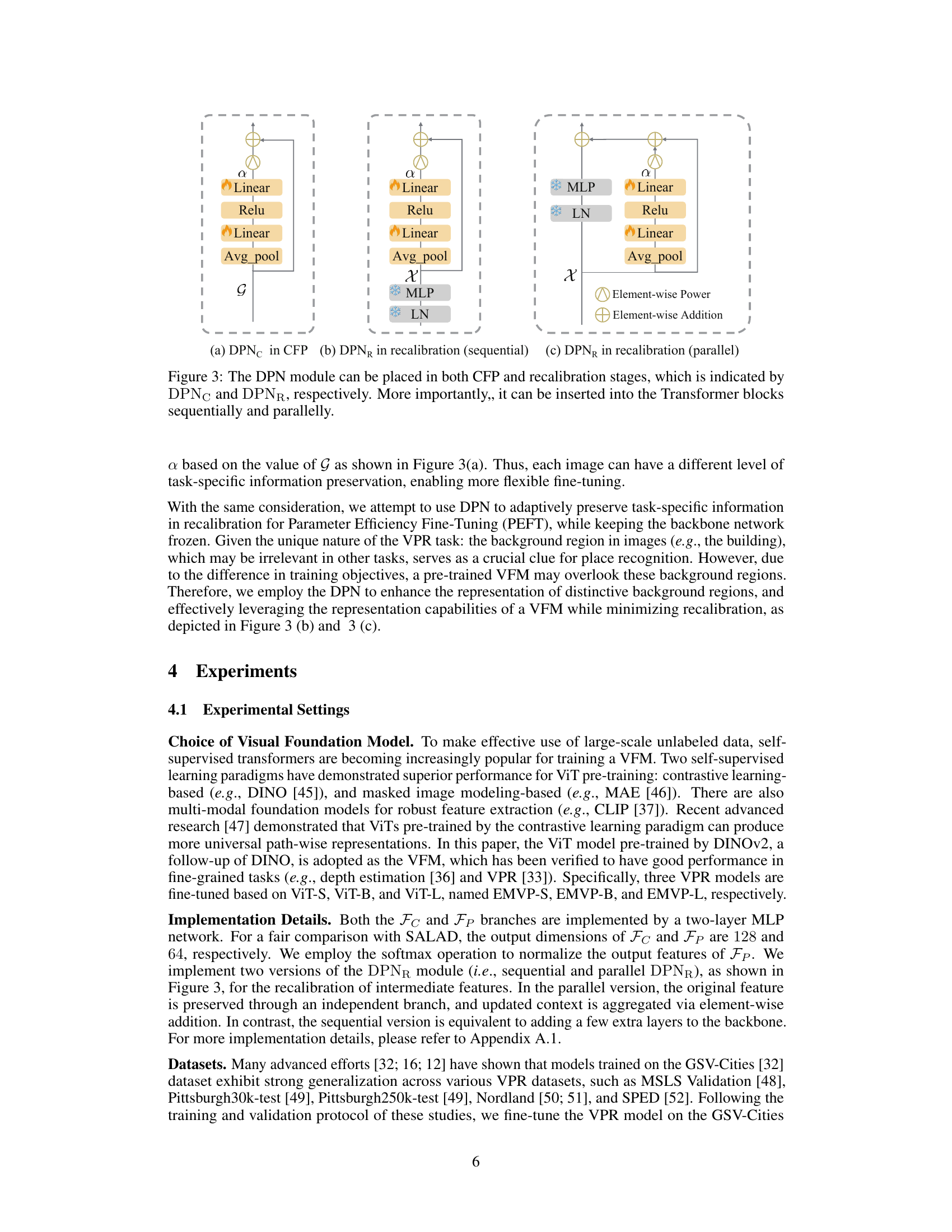
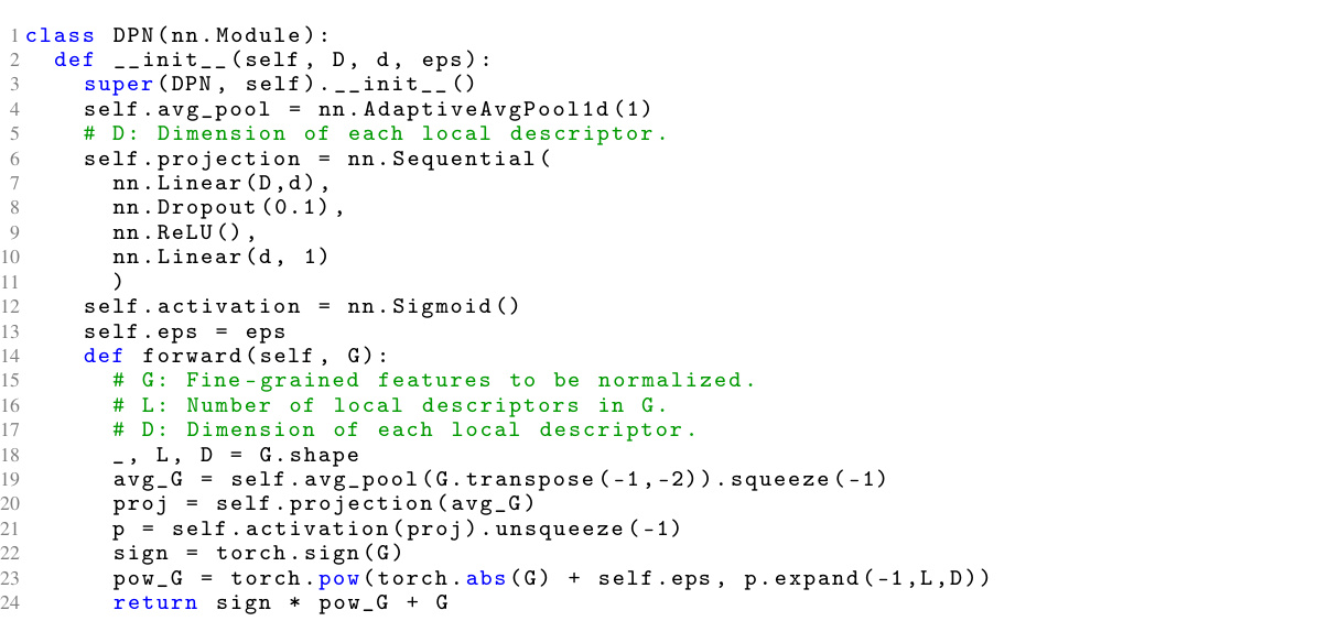
🔼 This figure shows three variations of the Dynamic Power Normalization (DPN) module. The DPN module is a key component of the EMVP pipeline, designed to adaptively control the preservation of task-specific information. The three variations illustrate its implementation in different stages of the pipeline: (a) DPNC in the Centroid-Free Probing (CFP) stage, (b) DPNR in the recalibration stage implemented sequentially, and (c) DPNR in recalibration implemented in parallel. The diagrams depict the architecture of each variation, highlighting the placement of the DPN module within the larger pipeline.
read the caption
Figure 3: The DPN module can be placed in both CFP and recalibration stages, which is indicated by DPNC and DPNR, respectively. More importantly,, it can be inserted into the Transformer blocks sequentially and parallelly.
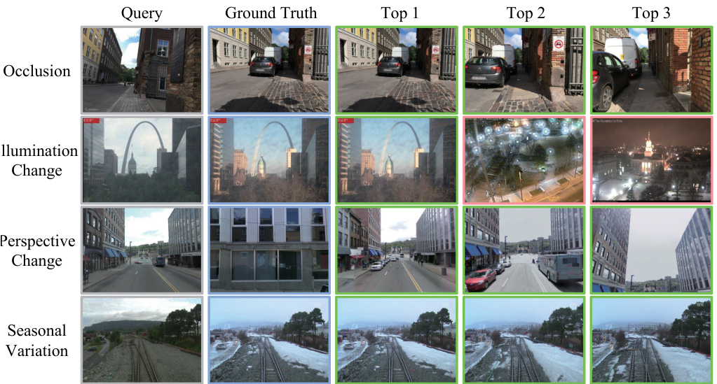
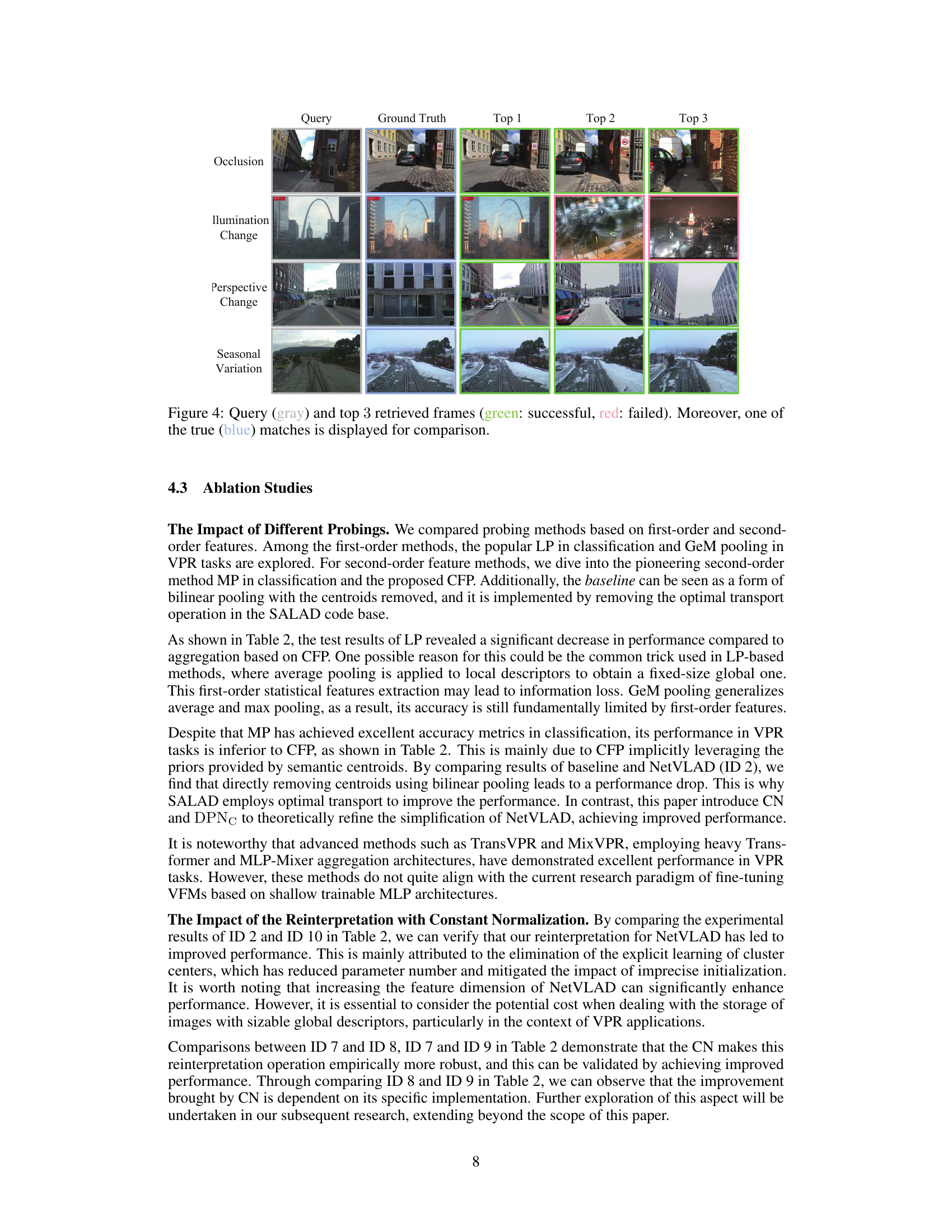
🔼 This figure shows examples of visual place recognition results under various challenging conditions. For each row, representing a different challenge (occlusion, illumination change, perspective change, and seasonal variation), the query image is shown alongside its ground truth match and the top three retrieved images from the model. Green indicates a successful match, red indicates a failed match, and blue (in some cases) shows another correct match. This visualization helps illustrate the model’s performance in handling these challenging scenarios, as well as the variety of challenges it is tested against.
read the caption
Figure 4: Query (gray) and top 3 retrieved frames (green: successful, red: failed). Moreover, one of the true (blue) matches is displayed for comparison.
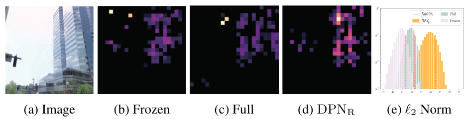
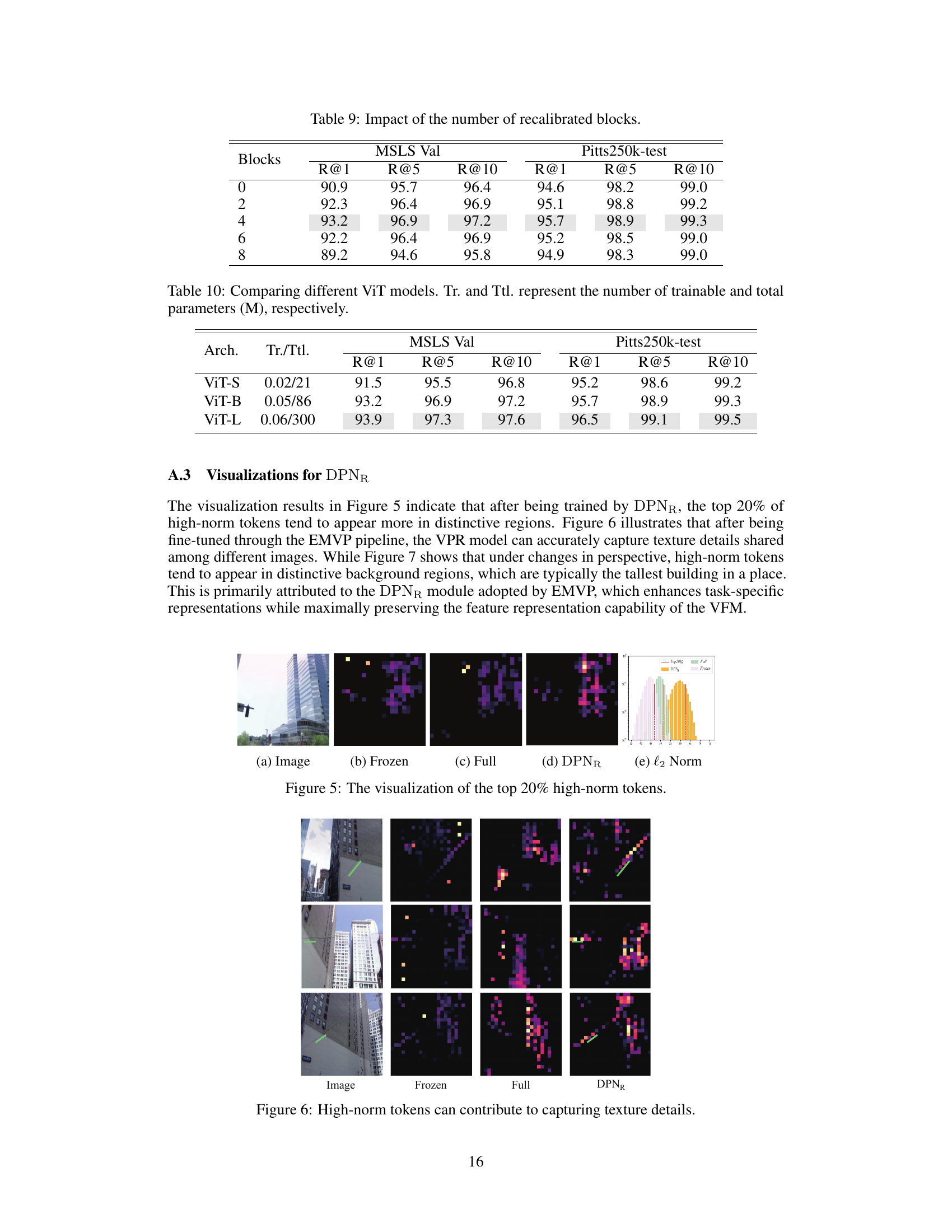
🔼 The figure visualizes the top 20% of high-norm tokens obtained from different model variations: frozen backbone, fully fine-tuned model, and model with the Dynamic Power Normalization (DPNR) module. It compares the distribution of high-norm tokens across different parts of the image, highlighting the impact of DPNR in focusing attention on specific regions relevant to visual place recognition. A histogram is included showing the distribution of high-norm token values for each variation.
read the caption
Figure 5: The visualization of the top 20% high-norm tokens.
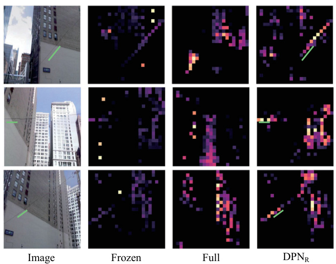
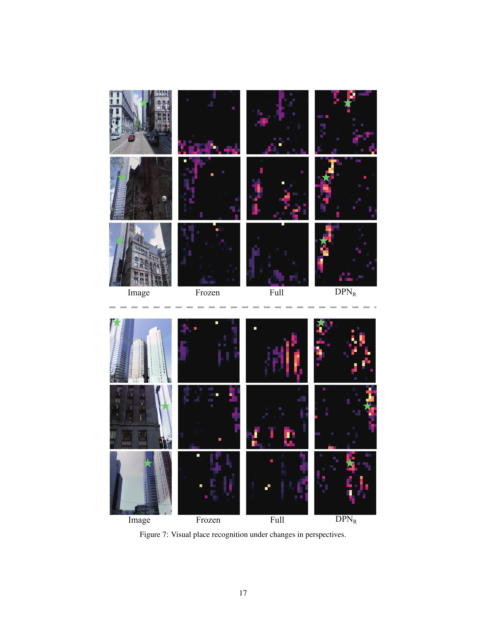
🔼 This figure shows the effectiveness of the proposed EMVP model in handling changes in perspectives. It displays the high-norm tokens for several images across different model variations: the original image, the frozen model, the fully fine-tuned model, and the model with DPNr. The results indicate that the EMVP model, particularly with the DPNr module, is able to maintain consistent focus on distinctive background features even when the viewpoint changes drastically.
read the caption
Figure 7: Visual place recognition under changes in perspectives.
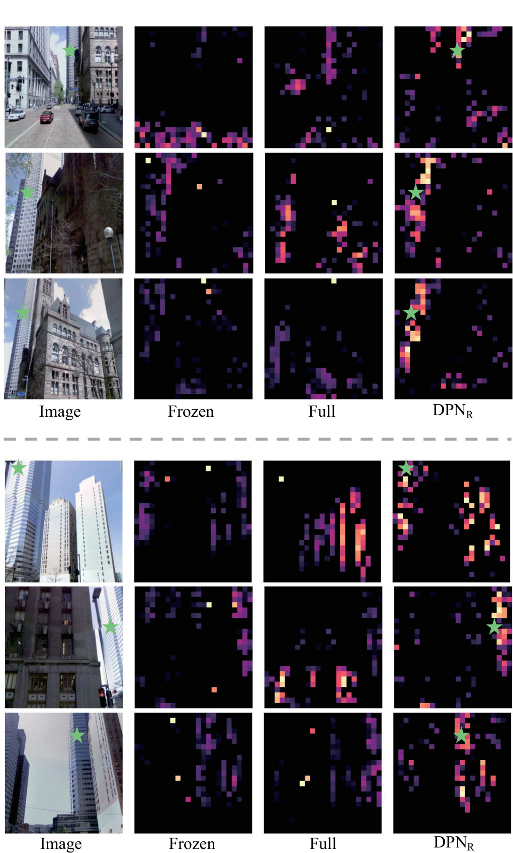
🔼 This figure shows the results of visual place recognition experiments under different perspectives. The top row shows the original images, followed by results from a model with a frozen backbone, a fully fine-tuned model, and a model using the proposed Dynamic Power Normalization (DPN) in the recalibration stage. The bottom row shows similar results but with different images and perspectives. The highlighted regions in the heatmap visualizations represent areas that the model is focusing on for place recognition. The green stars in the images indicate the ground truth locations.
read the caption
Figure 7: Visual place recognition under changes in perspectives.
More on tables
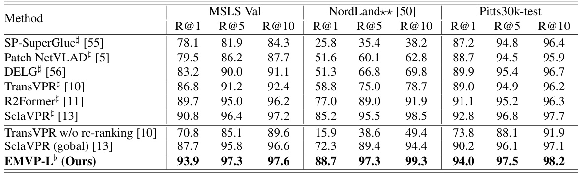
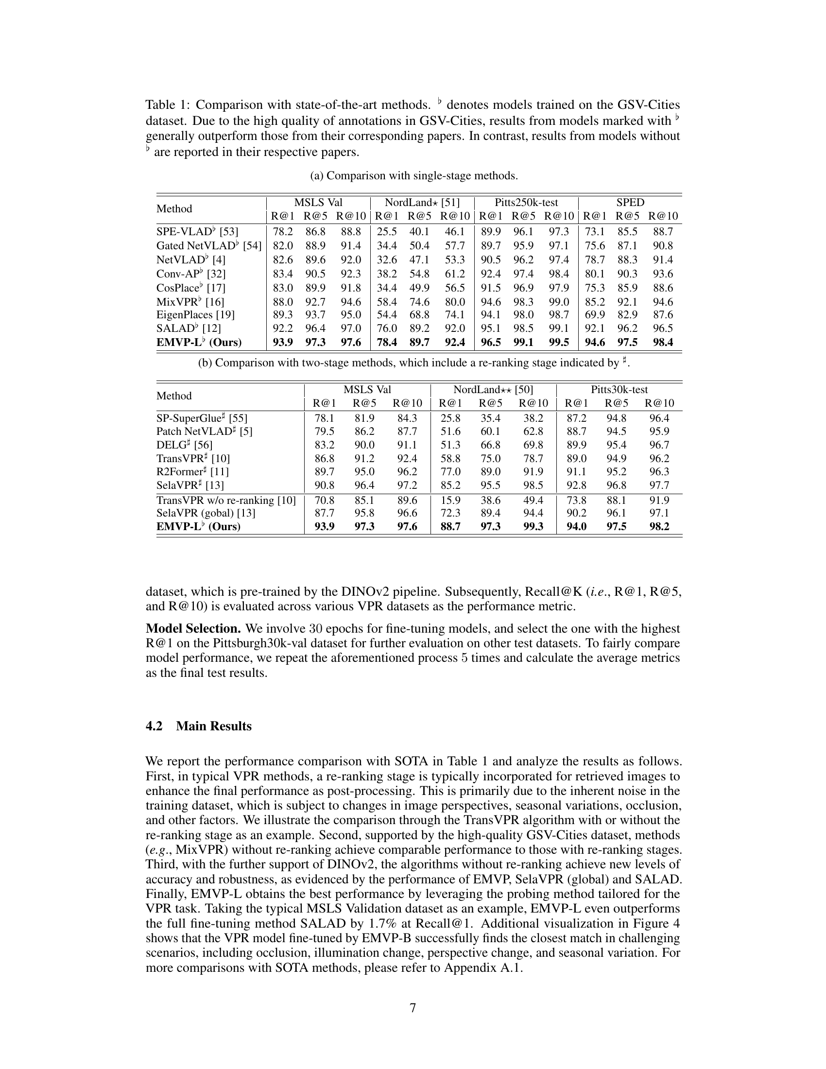
🔼 This table compares the EMVP model’s performance with other state-of-the-art visual place recognition (VPR) methods on four standard datasets: MSLS Validation, Nordland, Pitts250k-test, and SPED. The table is divided into two sections: single-stage methods and two-stage methods (those that also include a re-ranking stage). Recall@K (R@K) for K=1, 5, and 10 is reported as the performance metric, showing the percentage of times the correct image was retrieved within the top K ranked results. The table highlights the superior performance of EMVP-L (the EMVP model using the ViT-L architecture) compared to other methods, especially those without the re-ranking step.
read the caption
Table 1: Comparison with state-of-the-art methods. ♭ denotes models trained on the GSV-Cities dataset. Due to the high quality of annotations in GSV-Cities, results from models marked with ♭ generally outperform those from their corresponding papers. In contrast, results from models without ♭ are reported in their respective papers.
🔼 This table compares the proposed EMVP model’s performance with other state-of-the-art (SOTA) visual place recognition (VPR) methods across four benchmark datasets: MSLS Validation, Nordland, Pitts250k-test, and SPED. The comparison is done for single-stage and two-stage methods, and the table highlights the Recall@K (R@1, R@5, R@10) metric. The superscript ♭ indicates that the model was trained on the GSV-Cities dataset, which is known for its high annotation quality, leading to better results. The table effectively shows EMVP’s superior performance compared to existing methods.
read the caption
Table 1: Comparison with state-of-the-art methods. ♭ denotes models trained on the GSV-Cities dataset. Due to the high quality of annotations in GSV-Cities, results from models marked with ♭ generally outperform those from their corresponding papers. In contrast, results from models without ♭ are reported in their respective papers.
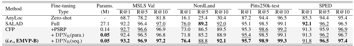
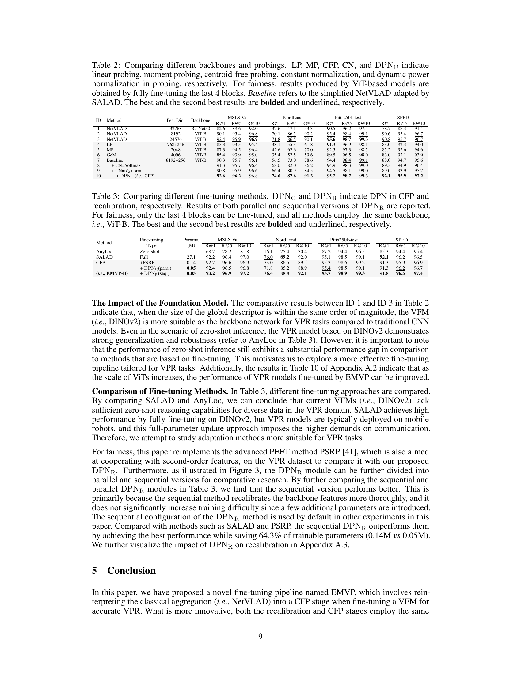
🔼 This table compares different fine-tuning methods for visual place recognition. It focuses on the impact of the Dynamic Power Normalization (DPN) module within the Centroid-Free Probing (CFP) stage and recalibration stage. Both parallel and sequential versions of DPN in the recalibration stage are evaluated. The table highlights the best performing methods while ensuring a fair comparison by using the same ViT-B backbone and only fine-tuning the last 4 blocks. The results (Recall@1, Recall@5, Recall@10) across the MSLS Validation, Nordland, Pittsburgh250k-test, and SPED datasets are shown, indicating the accuracy and efficiency of different methods.
read the caption
Table 3: Comparing different fine-tuning methods. DPNC and DPNR indicate DPN in CFP and recalibration, respectively. Results of both parallel and sequential versions of DPNR are reported. For fairness, only the last 4 blocks can be fine-tuned, and all methods employ the same backbone, i.e., ViT-B. The best and the second best results are bolded and underlined, respectively.
🔼 This table compares the proposed EMVP model’s performance with several state-of-the-art (SOTA) visual place recognition (VPR) methods on four benchmark datasets: MSLS Validation, NordLand, Pitts250k-test, and SPED. The table is divided into two sections: (a) compares EMVP with single-stage methods (methods without a re-ranking stage), and (b) compares EMVP with two-stage methods (methods that include a re-ranking stage). The results are presented as Recall@K (R@K) values where K = 1, 5, and 10, indicating the percentage of times the correct image is retrieved within the top K retrieved images.
read the caption
Table 1: Comparison with state-of-the-art methods. ♭ denotes models trained on the GSV-Cities dataset. Due to the high quality of annotations in GSV-Cities, results from models marked with ♭ generally outperform those from their corresponding papers. In contrast, results from models without ♭ are reported in their respective papers.
🔼 This table compares the proposed EMVP model’s performance with other state-of-the-art visual place recognition (VPR) methods across four datasets: MSLS Validation, Nordland, Pitts250k-test, and SPED. It reports Recall@K (R@K) values for K=1, 5, and 10, showing the percentage of correctly retrieved images within the top K retrieved images. The table is divided into two parts: single-stage methods and two-stage methods. Single-stage methods directly produce a ranking of images, while two-stage methods use a ranking step followed by a reranking step to refine the ranking. The high quality of annotations in the GSV-Cities dataset (used to train several models), allows for a fairer comparison of results reported by different papers. The table highlights EMVP’s superior performance.
read the caption
Table 1: Comparison with state-of-the-art methods. ♭ denotes models trained on the GSV-Cities dataset. Due to the high quality of annotations in GSV-Cities, results from models marked with ♭ generally outperform those from their corresponding papers. In contrast, results from models without ♭ are reported in their respective papers.
🔼 This table compares the proposed EMVP model’s performance with other state-of-the-art visual place recognition (VPR) methods on four benchmark datasets: MSLS Validation, NordLand, Pitts250k-test, and SPED. The results are presented as Recall@K (R@K) where K represents 1, 5, and 10, indicating the top K retrieved images. The table is divided into two sections: one comparing single-stage methods and another comparing two-stage methods that include a re-ranking stage. The table highlights that the EMVP model achieves superior performance compared to the other methods across all datasets.
read the caption
Table 1: Comparison with state-of-the-art methods. ♭ denotes models trained on the GSV-Cities dataset. Due to the high quality of annotations in GSV-Cities, results from models marked with ♭ generally outperform those from their corresponding papers. In contrast, results from models without ♭ are reported in their respective papers.
🔼 This table compares the proposed EMVP model’s performance with other state-of-the-art visual place recognition (VPR) methods across four benchmark datasets (MSLS Validation, NordLand, Pitts250k-test, and SPED). The results are presented in terms of Recall@K (R@1, R@5, R@10), showing the percentage of correctly retrieved images among the top 1, 5, and 10 retrieved images for each query image. The table also distinguishes between single-stage and two-stage methods, highlighting the impact of a re-ranking stage on performance. The use of the GSV-Cities dataset for training is noted as a factor influencing performance comparison.
read the caption
Table 1: Comparison with state-of-the-art methods. ♭ denotes models trained on the GSV-Cities dataset. Due to the high quality of annotations in GSV-Cities, results from models marked with ♭ generally outperform those from their corresponding papers. In contrast, results from models without ♭ are reported in their respective papers.
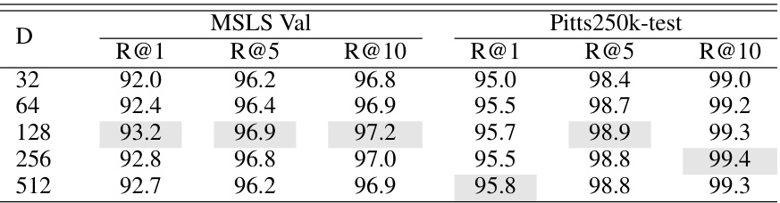
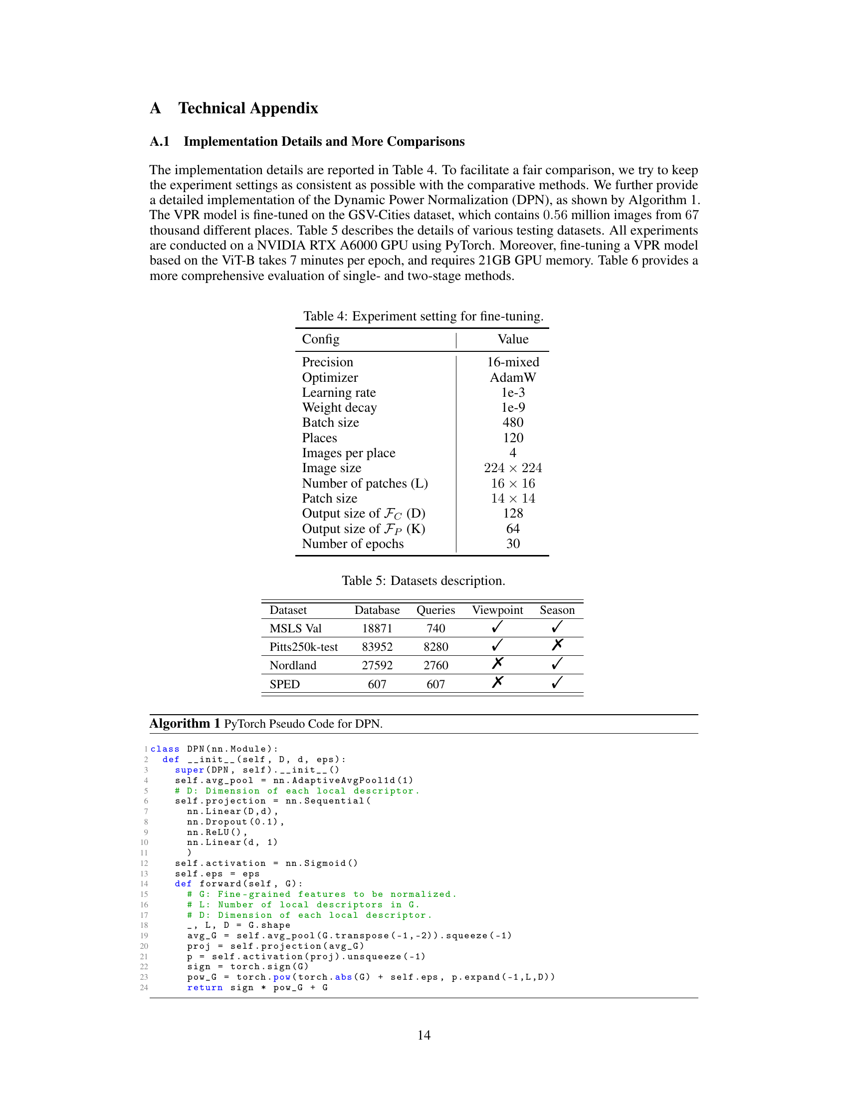
🔼 This table presents the ablation study on the output size of Fc (feature dimension) while keeping K (number of semantic centroids) constant at 64. It shows the Recall@1, Recall@5, and Recall@10 for the MSLS Validation and Pitts250k-test datasets with different values of D (dimension of Fc). This helps analyze the impact of the feature dimension on the performance of visual place recognition.
read the caption
Table 7: Impact of the output sizes of Fc (K = 64).
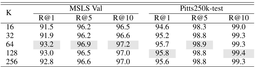
🔼 This table shows the impact of varying the output size of Fp (K) on the performance of the EMVP model, measured by Recall@1, Recall@5, and Recall@10 on the MSLS Validation and Pitts250k-test datasets. The dimension of Fc (D) is fixed at 128. The results suggest that the model’s performance is relatively stable across a range of K values.
read the caption
Table 8: Impact of the output sizes of Fp (D = 128).
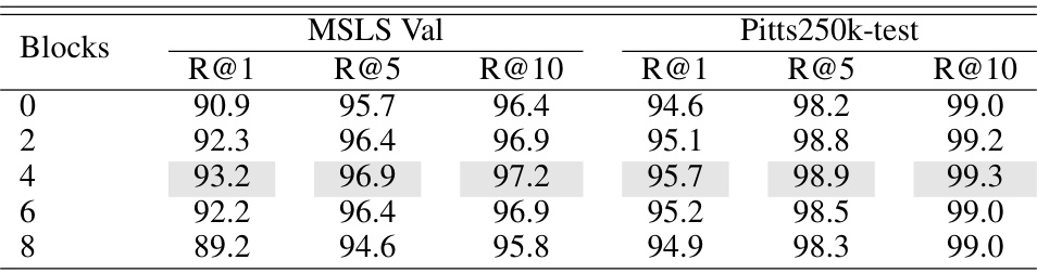
🔼 This table shows the impact of the number of recalibrated blocks on the performance of the EMVP model. The model is evaluated using Recall@1, Recall@5, and Recall@10 metrics on the MSLS Validation and Pitts250k-test datasets. The results show that recalibrating the features in the last 4 blocks leads to the best performance, suggesting that focusing the fine-tuning on specific layers of the network is beneficial for improving the accuracy and efficiency of the VPR model. Recalibrating fewer or more blocks results in lower performance.
read the caption
Table 9: Impact of the number of recalibrated blocks.
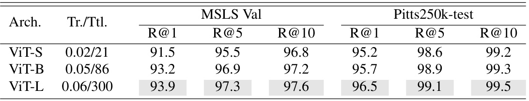
🔼 This table compares the performance of different sized Vision Transformer (ViT) models (ViT-S, ViT-B, ViT-L) on two Visual Place Recognition (VPR) datasets (MSLS Validation and Pitts250k-test). The results are shown as Recall@K (R@1, R@5, R@10). The table also lists the number of trainable and total parameters (in millions) for each model, indicating the model’s size and complexity.
read the caption
Table 10: Comparing different ViT models. Tr. and Ttl. represent the number of trainable and total parameters (M), respectively.
Full paper#