↗ OpenReview ↗ NeurIPS Homepage ↗ Chat
TL;DR#
The research addresses the challenge of making predictions in machine learning when there is significant uncertainty. This is crucial in many real-world applications, such as medicine and self-driving cars, where uncertainty needs to be quantified. Current methods often struggle to adequately represent uncertainty, particularly in situations with ambiguous data where different annotations exist for the same instance. The paper also highlights that existing machine learning methods may inadequately capture uncertainty, especially epistemic uncertainty.
To address these issues, the paper proposes a new approach that combines conformal prediction with credal sets. Conformal prediction provides rigorous mathematical guarantees for the validity of predictions, while credal sets offer a flexible way to represent uncertainty. Experiments on several datasets show that this novel method produces valid credal sets, effectively capturing both types of uncertainty. The results demonstrate that the approach is both effective and reliable in situations with high uncertainty, offering strong potential for improving the robustness of machine learning models in various real-world applications.
Key Takeaways#
Why does it matter?#
This paper is important because it presents a novel method for making predictions in machine learning that accounts for both aleatoric and epistemic uncertainty. This is crucial in situations where uncertainty is high, such as medical diagnosis or autonomous driving. The method uses conformal prediction, which provides strong theoretical guarantees, and it’s shown to be effective on various tasks. This work opens up new avenues of research by connecting machine learning with imprecise probability theory, leading to more robust and reliable predictions.
Visual Insights#

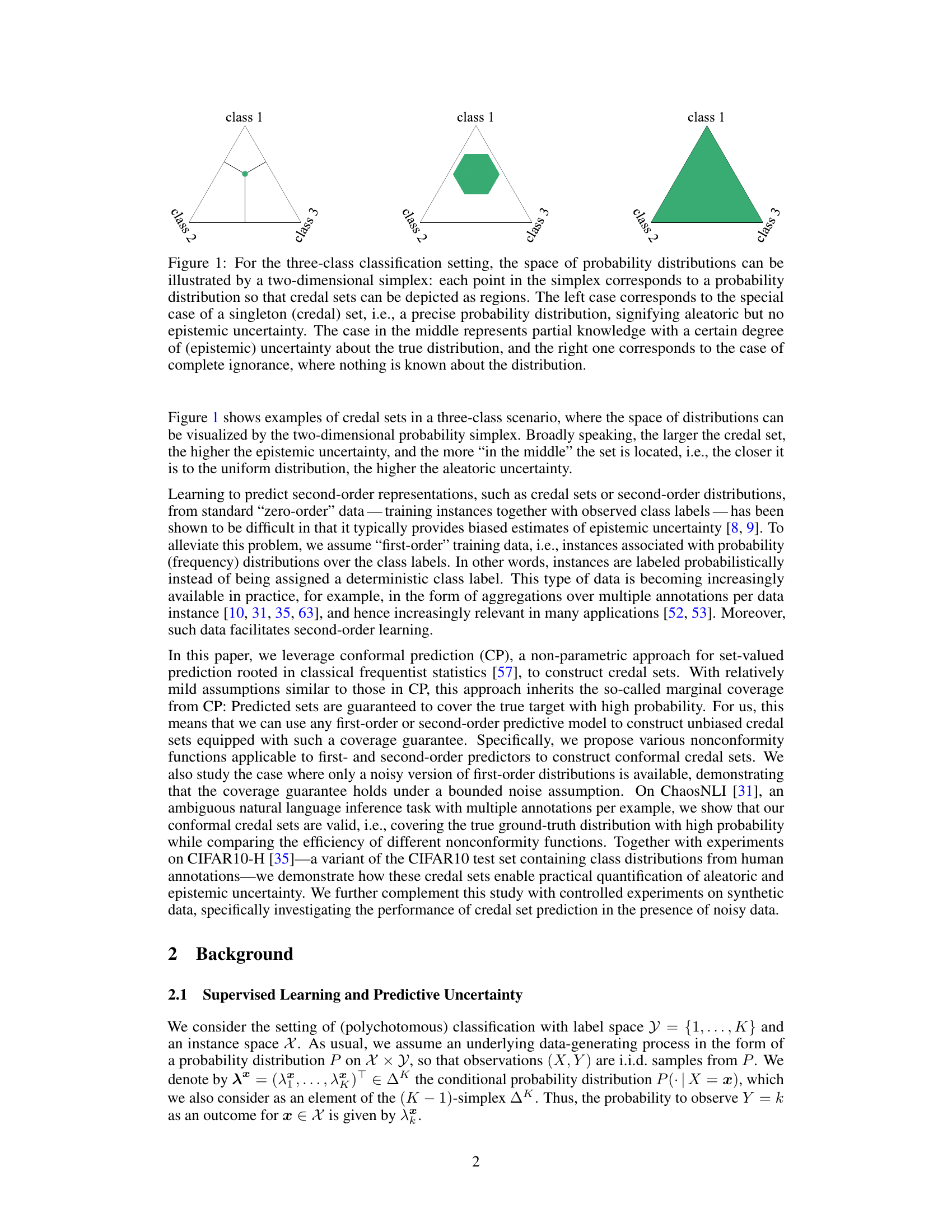
This figure illustrates how credal sets are represented in a three-class classification problem. The space of all possible probability distributions is shown as a 2D simplex (triangle). A single point represents a precise probability distribution (no epistemic uncertainty, only aleatoric), while regions within the simplex depict credal sets (sets of probability distributions representing both aleatoric and epistemic uncertainty). The size and location of the credal set within the simplex indicate the degree of uncertainty. The leftmost image shows a singleton (precise probability), the middle shows partial knowledge, and the rightmost represents complete ignorance.
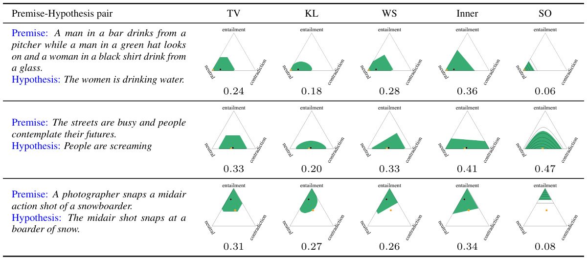
This figure displays credal sets generated by different methods (TV, KL, WS, Inner, SO) for three example instances from the ChaosNLI dataset. Orange squares represent the ground truth probability distributions, while black circles show predictions from first-order learners (TV, KL, WS, Inner). The last column illustrates predictions using a second-order learner via contour plots. The miscoverage rate is set to α=0.2, and the efficiency of each prediction (how small the set is) is noted below each visualization.
In-depth insights#
Credal Set Prediction#
Credal set prediction presents a novel approach to uncertainty quantification in machine learning. Instead of predicting a single point estimate, it predicts a set of probability distributions, representing both aleatoric and epistemic uncertainty. This approach is particularly useful in scenarios with ambiguous or noisy data, where a single prediction might be misleading. Conformal prediction is leveraged to construct these credal sets, guaranteeing validity with high probability without strong distributional assumptions. The method involves training a predictive model (first-order or second-order) and using a nonconformity function to quantify the strangeness of data points. This approach is shown to be effective in scenarios with first-order (probabilistically labeled) data, offering improved uncertainty quantification and a more robust approach to classification and prediction tasks. However, limitations exist, notably the reliance on first-order data and the computational challenges associated with high-dimensional data and multiple classes. Future research could explore the generalization to zero-order data and more efficient algorithms for larger-scale problems.
Conformal Prediction#
Conformal prediction is a powerful nonparametric approach for generating prediction sets with guaranteed validity. It’s particularly valuable when dealing with uncertainty, as it doesn’t rely on strong distributional assumptions. The core idea is to quantify the “strangeness” of a data point relative to a calibration set, using a nonconformity measure. This allows for the construction of prediction sets that contain the true value with a user-specified probability, regardless of the underlying data distribution. This makes conformal prediction robust and widely applicable, especially in settings where the assumptions of traditional methods are violated. However, efficiency can be a concern, as the size of the prediction sets can be large, reducing the accuracy of point estimates. Despite this limitation, its theoretical guarantees and adaptability make it a valuable tool for various machine learning tasks, especially when uncertainty quantification is crucial.
Uncertainty Quantification#
The concept of uncertainty quantification is central to the research paper, focusing on how to represent and manage uncertainty in machine learning predictions. The authors address this challenge by leveraging credal sets, which are sets of probability distributions representing both aleatoric (inherent randomness) and epistemic (knowledge limitations) uncertainty. The paper proposes using conformal prediction to construct these credal sets, offering validity guarantees without strong distributional assumptions. This approach is further extended to handle noisy or imprecise training data, providing a robust and practical method for uncertainty quantification in various classification settings. Ambiguous classification tasks serve as key applications, demonstrating the method’s utility in quantifying uncertainty from multiple sources. The paper also explores different nonconformity functions and investigates the performance in separating and quantifying aleatoric and epistemic components of uncertainty. Ultimately, the work showcases the potential of the proposed approach for generating reliable, uncertainty-aware machine learning predictions.
Noisy Data Handling#
The paper addresses the crucial issue of noisy data in the context of credal set prediction. It acknowledges that real-world data often deviates from ideal conditions, particularly with probabilistic labels derived from multiple human annotators. The authors recognize the limitations of assuming perfectly precise probability distributions and introduce a bounded noise assumption to account for this imperfection. This assumption allows them to formally adapt their conformal prediction method to maintain validity guarantees even in the presence of noisy labels, ensuring that predicted credal sets still cover the true distribution with high probability. Robustness under noisy data is experimentally demonstrated through controlled studies on synthetic data and real-world applications. The approach involves modifying the miscoverage rate in the conformal prediction framework to account for the noise level, allowing for principled uncertainty quantification even with imperfect data.
Future Research#
The paper’s ‘Future Research’ section would benefit from exploring several avenues. Extending the conformal credal set prediction to standard (zero-order) data is crucial, as first-order data isn’t always available. Investigating different nonconformity functions that provide closed-form solutions for credal sets or improved efficiency and reduced uncertainty is vital. Constructing label sets from credal sets presents an exciting opportunity to potentially provide richer information compared to standard conformal prediction. Finally, a more detailed investigation into handling noisy data, especially exploring the impact of different noise models and developing more robust methods, is necessary. The impact of high-dimensional data on the efficiency and scalability of the approach also requires further investigation. Considering the broader implications of the work, specifically focusing on how to best handle uncertainty in safety-critical applications, will increase its real-world value.
More visual insights#
More on figures

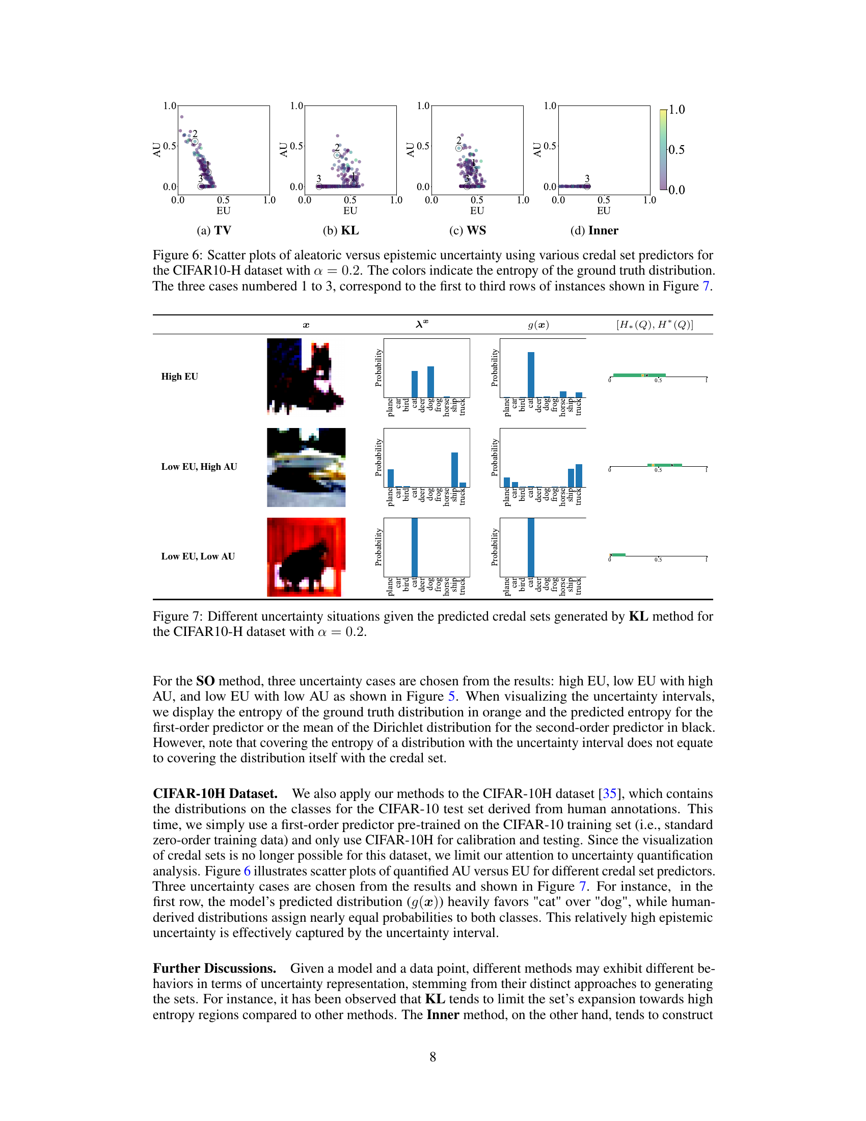
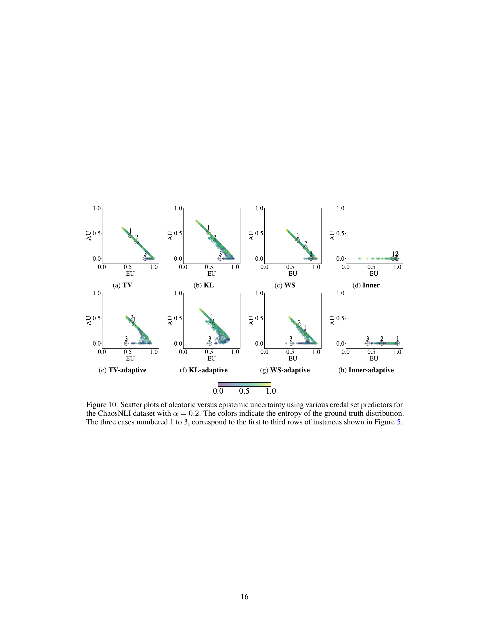
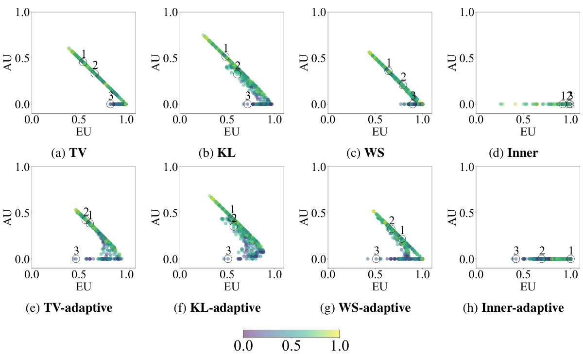
This figure shows scatter plots visualizing the relationship between aleatoric and epistemic uncertainty for different credal set predictors on the ChaosNLI dataset. Each point represents a data instance, with its x-coordinate representing the epistemic uncertainty and its y-coordinate representing the aleatoric uncertainty. The color of the point reflects the entropy of the corresponding ground truth distribution. Three specific cases from Figure 5 are highlighted, illustrating various uncertainty scenarios. The results demonstrate the capability of the proposed methodology to disentangle and quantify both aleatoric and epistemic uncertainties.

This figure shows examples of credal sets generated for three different instances from the ChaosNLI dataset using both first-order and second-order prediction models. The orange squares represent the true underlying probability distributions, while black circles show the predictions made by the model(s). In the first four columns, first-order models are used. In the last column, a second-order model is used, shown as contour plots. The efficiency of each credal set is shown below its corresponding visualization. The value α = 0.2 represents the target miscoverage rate (i.e., the probability that the true distribution is not contained within the credal set).
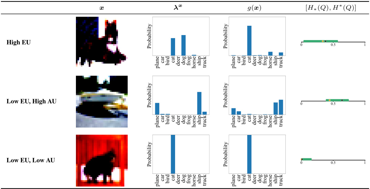
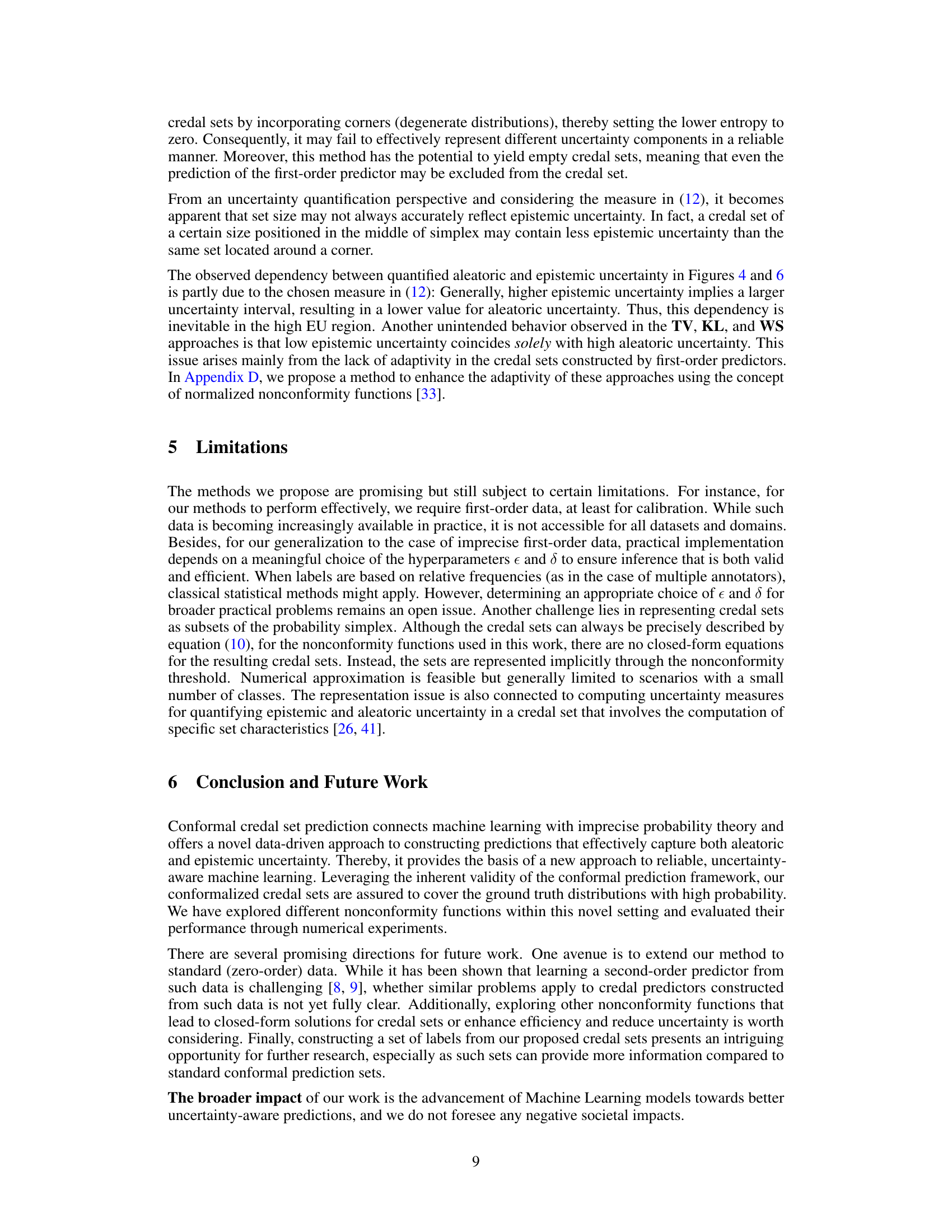
This figure shows three examples from the CIFAR10-H dataset illustrating different uncertainty situations. Each row represents a different uncertainty scenario: high epistemic uncertainty (High EU), low epistemic uncertainty with high aleatoric uncertainty (Low EU, High AU), and low epistemic uncertainty with low aleatoric uncertainty (Low EU, Low AU). For each scenario, the image (x), the ground truth probability distribution (λx), the model’s prediction (g(x)), and the uncertainty interval [H*(Q), H*(Q)] are displayed. The uncertainty intervals visually represent the range of plausible probability distributions for the given input, reflecting the level of uncertainty in the model’s prediction.

This figure provides a visual representation of the ChaosNLI and CIFAR10-H datasets used in the paper. Panel (a) shows a scatter plot of the ChaosNLI dataset, illustrating the distribution of probability distributions across the three classes (entailment, neutral, contradiction). Panels (b) and (c) display histograms of the entropy values for ChaosNLI and CIFAR10-H, respectively, offering insights into the level of uncertainty in each dataset. The x-axis represents entropy values, ranging from 0 to 1, with higher entropy indicating greater uncertainty, and the y-axis shows the frequency of instances with a given entropy level.

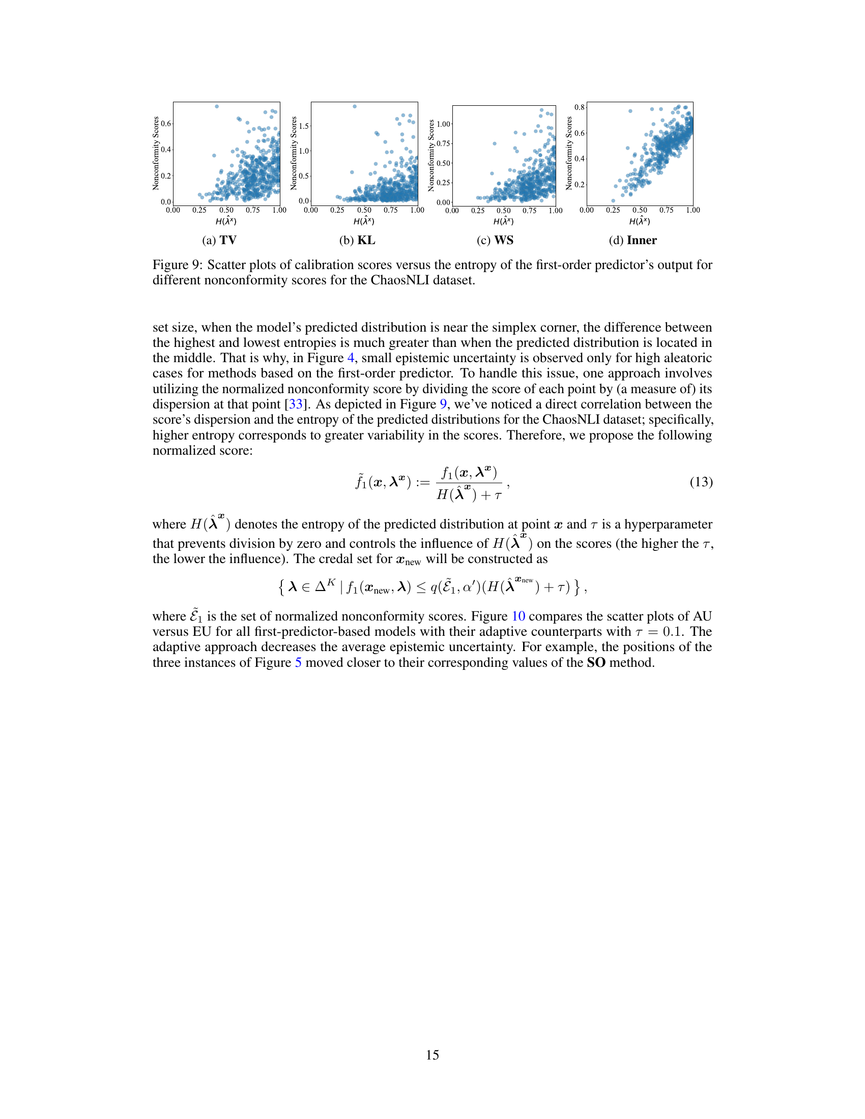
The figure shows four scatter plots, one for each of the four nonconformity functions used in the paper (Total Variation, Kullback-Leibler divergence, Wasserstein distance, and Inner product). Each plot displays the relationship between the calibration scores (y-axis) and the entropy of the predicted distribution (x-axis) for the ChaosNLI dataset. The plots help to visualize the performance of each nonconformity function during the calibration phase of conformal prediction. The spread of points and their distribution provide insights into how well each function differentiates between more and less ’normal’ data points based on their predicted distributions.
This figure displays credal sets predicted by different models for three example instances from the ChaosNLI dataset. Each example is represented visually using a probability simplex (triangle). The true distribution for each instance is shown as an orange square. The first four columns illustrate the results from four different first-order prediction models using different methods of calculating nonconformity. Each model’s prediction is shown as a black circle. The last column shows the result from a second-order model, represented as a contour plot indicating a range of probability distributions within the simplex. The caption explains that the miscoverage rate used was 0.2 and shows the calculated efficiency for each prediction.
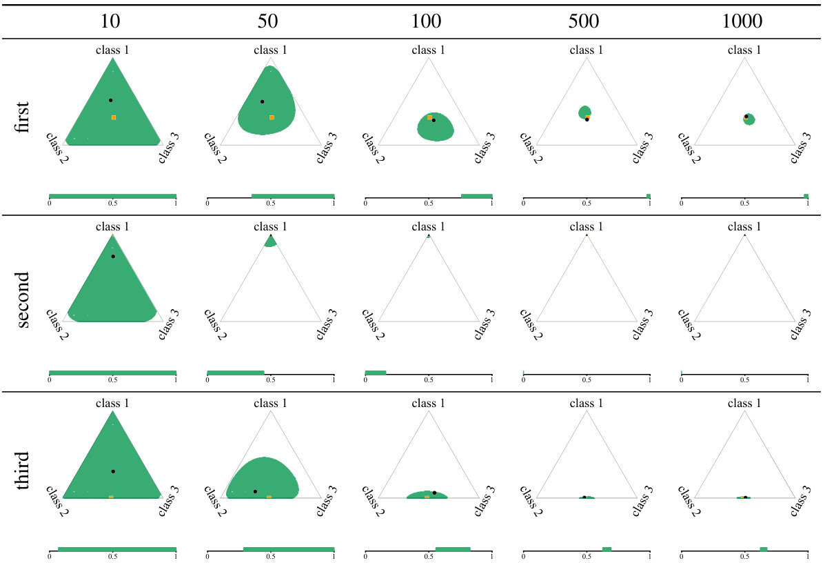
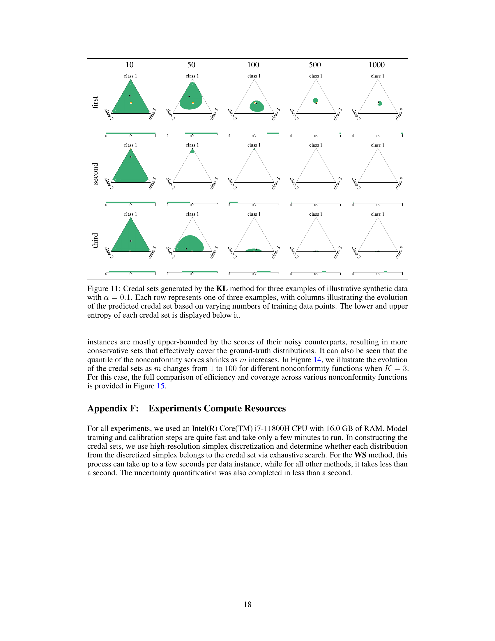
This figure shows the evolution of credal sets generated using the KL method on three different examples of synthetic data as the number of training data points increases. Each row represents one of the three examples, and the columns show how the credal set changes. The lower and upper entropy values are displayed below each credal set to help quantify the uncertainty.
This figure visualizes credal sets predicted by different models for three example instances from the ChaosNLI dataset. The ground truth probability distributions are shown as orange squares. The first four columns display predictions from first-order models, represented as black circles. The final column shows predictions from a second-order model, visualized as contour plots. The figure highlights the variation in credal set size and shape across different prediction methods, indicating different levels of uncertainty. The miscoverage rate (α) is fixed at 0.2, and each credal set’s efficiency is shown below it.

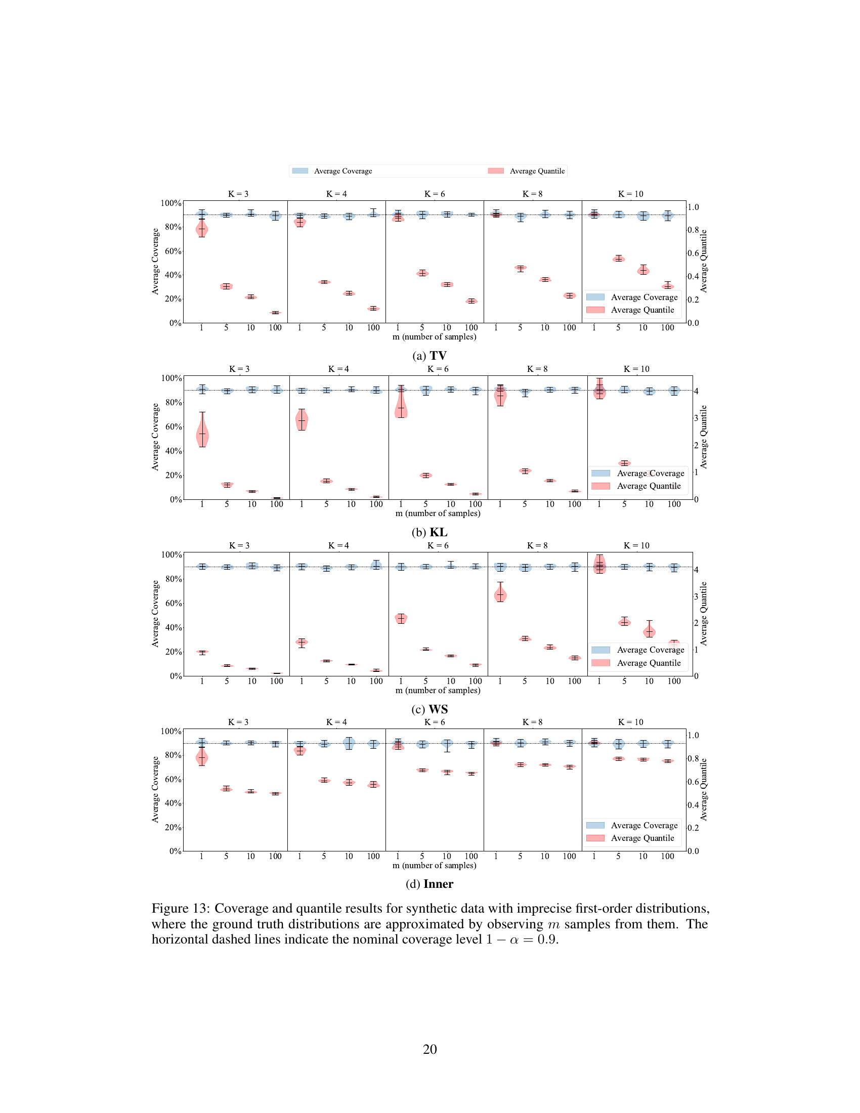
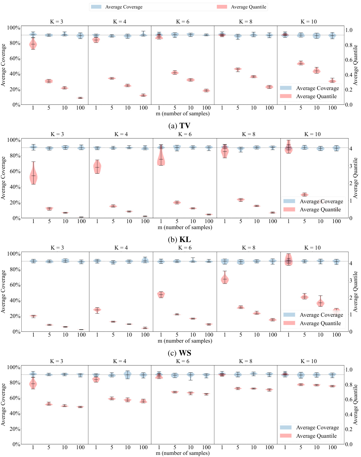
This figure shows the results of an experiment on synthetic data to evaluate the performance of different nonconformity functions used in conformal credal set prediction. The experiment uses imprecise first-order data, meaning that the true probability distributions are approximated by sampling. The figure presents violin plots illustrating the average coverage and efficiency of different nonconformity functions (TV, KL, WS, Inner, SO) across various miscoverage rates (α) and different numbers of samples (m) used to approximate the distributions. The horizontal dashed lines represent the nominal coverage levels, which are the desired lower bounds of coverage. The plots show how coverage and efficiency vary with the nonconformity function, miscoverage rate, and the number of samples used in the approximations.
More on tables

This figure shows the results of an experiment evaluating different nonconformity functions for constructing conformal credal sets using synthetic data with imprecise first-order distributions. The experiment is performed with K=3 classes. The plot displays the average coverage and efficiency of different methods across various miscoverage rates (α). Horizontal dashed lines represent the nominal coverage level (1-α). The results help to assess the performance and validity of different nonconformity functions in the context of uncertain data.

This figure shows three examples from the ChaosNLI dataset to illustrate different uncertainty situations. Each row represents a different example, categorized as High Epistemic Uncertainty (EU), Low EU with High Aleatoric Uncertainty (AU), and Low EU with Low AU. The figure displays the predicted credal sets (using the SO method) in the form of a 2D simplex, visualizing the probability distribution across three classes: entailment, contradiction, and neutral. The orange square indicates the ground truth distribution, while the black circles represent the model predictions (for first-order predictors) or contour plots for the second-order predictor. The uncertainty intervals [H*(Q), H*(Q)] are also shown, representing the range of uncertainty from aleatoric and epistemic sources.

This table presents the results of an experiment evaluating the performance of different nonconformity functions in a setting with imprecise first-order data. The experiment varied the number of samples used to approximate the ground truth distributions (m) and the number of classes (K). The table shows the average coverage and quantiles of the nonconformity scores for different values of m and K, illustrating the robustness of the approach across various conditions. The nominal coverage level of 0.9 provides a baseline for assessing the quality of the method under different levels of noise.

This table displays the credal sets generated by different methods (TV, KL, WS, Inner, SO) for a single example from synthetic data with varying levels of noise in the first-order distributions. The number of samples used to approximate each distribution is shown in each row. The ground truth distribution is shown as an orange square, noisy versions of the distribution as red squares, first-order model predictions as black circles, and second-order model predictions as contour plots. The table illustrates the effect of different nonconformity functions and noise levels on the resulting credal sets.
Full paper#
