Spiking Graph Neural Network on Riemannian Manifolds

VKt0K3iOmO

Li Sun et el.

TL;DR
#

Traditional graph neural networks (GNNs) suffer from high computational costs and energy consumption. Spiking GNNs, inspired by the brain’s energy efficiency, offer a promising alternative, but existing models primarily focus on Euclidean spaces and face challenges with high latency during training. This paper addresses these limitations by developing a novel Manifold-valued Spiking GNN (MSG) that operates on Riemannian manifolds, thereby capturing the inherent geometric properties of graph data.

The MSG utilizes a newly designed spiking neuron which incorporates structural information into spike trains through graph convolution. Unlike prior approaches, MSG employs ‘Differentiation via Manifold’, an alternative training method that avoids the limitations of backpropagation. This method replaces the traditional back-propagation-through-time (BPTT) with a novel technique that is recurrence-free and computationally efficient. Theoretical analysis shows that MSG approximates a solver of manifold ordinary differential equations, providing a strong theoretical foundation. Experimental results demonstrate MSG’s superior performance and energy efficiency compared to existing spiking GNNs and traditional GNNs on various datasets.

Key Takeaways
#

Why does it matter?
#

This paper is crucial for researchers in graph neural networks and machine learning because it bridges the gap between energy-efficient spiking neural networks and the geometric properties of graph data represented by Riemannian manifolds. It offers a novel training method that significantly improves upon existing limitations, paving the way for more efficient and powerful graph learning models. This opens avenues for further research into manifold-valued neural networks and their applications to complex real-world problems.

Visual Insights
#

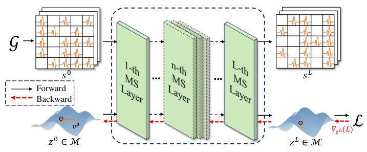
🔼 This figure illustrates the architecture of the Manifold-valued Spiking GNN (MSG). The input is a graph G represented as spike trains S⁰. These spike trains are processed by multiple Manifold Spiking Layers (MS Layers). Each MS Layer contains a Graph Convolutional Network (GCN) and a Manifold Spiking Neuron. The GCN incorporates structural information from the graph into the spike trains. The Manifold Spiking Neuron emits new spike trains and updates manifold representations using a diffeomorphism and exponential map. This process repeats across multiple layers, resulting in the final manifold representation Z^L and spike trains S^L, which are then used for downstream tasks. The red dashed line represents the proposed Differentiation via Manifold (DvM) approach, avoiding the high latency associated with Backpropagation-Through-Time (BPTT).
read the caption
Figure 1: MSG conducts parallel forwarding and enables a new training algorithm alleviating the high latency issue.

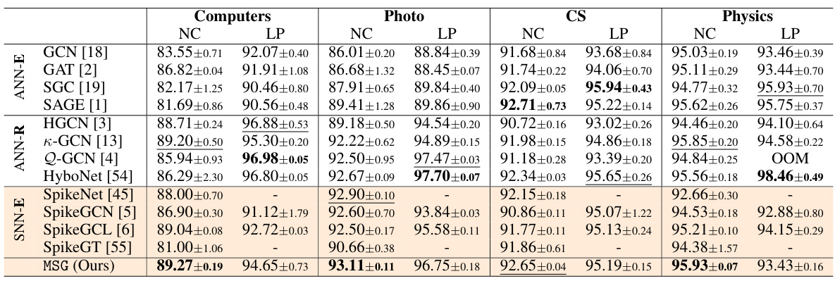
🔼 This table presents a comparison of different graph neural network (GNN) models’ performance on node classification and link prediction tasks. Four datasets (Computers, Photo, CS, Physics) are used. The table shows classification accuracy and AUC (Area Under the Curve) scores for each model and dataset. The best-performing model for each task and dataset is shown in bold, while the second-best is underlined. The results highlight the relative performance of various GNN architectures (ANN-based Euclidean, ANN-based Riemannian, and SNN-based Euclidean), illustrating the effectiveness and efficiency of different approaches.
read the caption
Table 1: Node Classification (NC) in terms of classification accuracy (%) and Link Prediction in terms of AUC (%) on Computers, Photo, CS and Physics datasets. The best results are boldfaced, and the runner-ups are underlined.

In-depth insights
#

Riemannian SNNs
#

Riemannian SNNs represent a significant advancement in neural network research, combining the energy efficiency of spiking neural networks (SNNs) with the ability of Riemannian geometry to handle complex, non-Euclidean data structures. This approach directly addresses limitations of traditional SNNs, which often struggle with data that cannot be easily embedded into Euclidean space. By leveraging Riemannian manifolds, these networks can naturally model data with inherent hierarchical or non-linear relationships, like those found in graph data. The key innovation lies in the development of new spiking neuron models that operate directly on Riemannian manifolds and enable efficient backpropagation through time. This avoids the computational burden and high latency often associated with surrogate gradients used in conventional SNNs. The theoretical underpinnings of Riemannian SNNs often involve elegant mathematical formulations, including diffeomorphisms and geodesic flows, to ensure robust and efficient learning. The potential applications of Riemannian SNNs are broad, ranging from graph neural networks for complex data analysis to more energy-efficient hardware implementations of artificial intelligence systems. However, challenges remain in developing efficient algorithms and optimizing the training process, especially for high-dimensional manifolds. Further research in this field could significantly impact various areas of machine learning and neuroscience.

Manifold Spiking
#

The concept of “Manifold Spiking” blends two distinct fields: the geometry of Riemannian manifolds and the dynamics of spiking neural networks (SNNs). It suggests representing and processing information within the complex, non-Euclidean spaces of manifolds, using the energy-efficient and biologically plausible communication method of SNNs. This approach presents several advantages: increased representational power by capturing the inherent geometric relationships of data, improved energy efficiency due to SNN’s inherent low-power operation, and potentially novel computational capabilities. However, it also poses significant challenges. The non-differentiable nature of spikes in SNNs requires novel training algorithms, and implementing operations within manifolds necessitates sophisticated mathematical techniques. Therefore, “Manifold Spiking” research would likely focus on designing new neuron models suitable for manifold spaces, developing efficient training methods (possibly bypassing backpropagation), and exploring applications where the inherent geometry of the data is crucial.

DvM Training
#

The proposed DvM (Differentiation via Manifold) training method presents a novel approach to address the limitations of traditional backpropagation methods in spiking neural networks (SNNs). Unlike conventional BPTT (Backpropagation Through Time) which suffers from high latency due to its recurrent nature, DvM leverages the geometric properties of Riemannian manifolds to enable a more efficient and direct computation of gradients. By decoupling the forward and backward passes, and employing the concept of diffeomorphism, DvM avoids the time-consuming iterative calculations of BPTT, leading to significantly faster training times. The theoretical foundation of DvM is rooted in differential geometry, particularly in the concepts of pullback and pushforward, ensuring the method’s rigorousness. This allows the replacement of the non-differentiable spike trains with differentiable manifold representations, simplifying the gradient computation. The resulting algorithm showcases superior performance compared to existing spiking GNN training techniques, with improvements in both accuracy and energy efficiency.

MSG Neural ODE
#

The heading ‘MSG Neural ODE’ suggests a novel approach that merges Manifold-valued Spiking GNNs (MSGs) with the framework of neural ordinary differential equations (ODEs). This implies a significant departure from traditional GNNs. Instead of discrete graph convolutions, the model likely uses continuous-time dynamics described by ODEs on Riemannian manifolds. This could provide improved expressiveness for modeling complex relationships in non-Euclidean graph data. The spiking aspect suggests an energy-efficient architecture, capitalizing on the biological inspiration of SNNs. The Riemannian manifold setting addresses the limitation of Euclidean-space GNNs by incorporating geometric information inherent in graph structures, enabling better handling of hierarchical or hyperbolic relationships often present in real-world networks. Combining this with the ODE framework offers a powerful tool for modeling dynamic processes on graphs. This approach’s theoretical underpinnings potentially involve rigorous mathematical analysis and could lead to more stable and efficient training algorithms. However, this sophistication may also present challenges in terms of computational cost and model interpretability.

Future Works
#

Future work could explore extending the Manifold-valued Spiking GNN (MSG) to handle dynamic graphs, a significant challenge in current spiking neural network research. This would involve adapting the model to process evolving graph structures and relationships, which could lead to breakthroughs in applications with dynamic data streams. Another promising avenue is investigating the performance of MSG on larger-scale, real-world graphs. Scaling the model efficiently remains a crucial aspect of practical application. Furthermore, research into different Riemannian manifolds beyond those already considered could uncover improved model performance for specific graph topologies and relationship types. The use of different spiking neuron models should also be investigated to better understand the trade-offs between model complexity, computational cost, and accuracy. Finally, exploring the implications of MSG’s theoretical connections to manifold ordinary differential equations (ODEs) for advanced model design and interpretation warrants further investigation.

More visual insights
#

More on figures

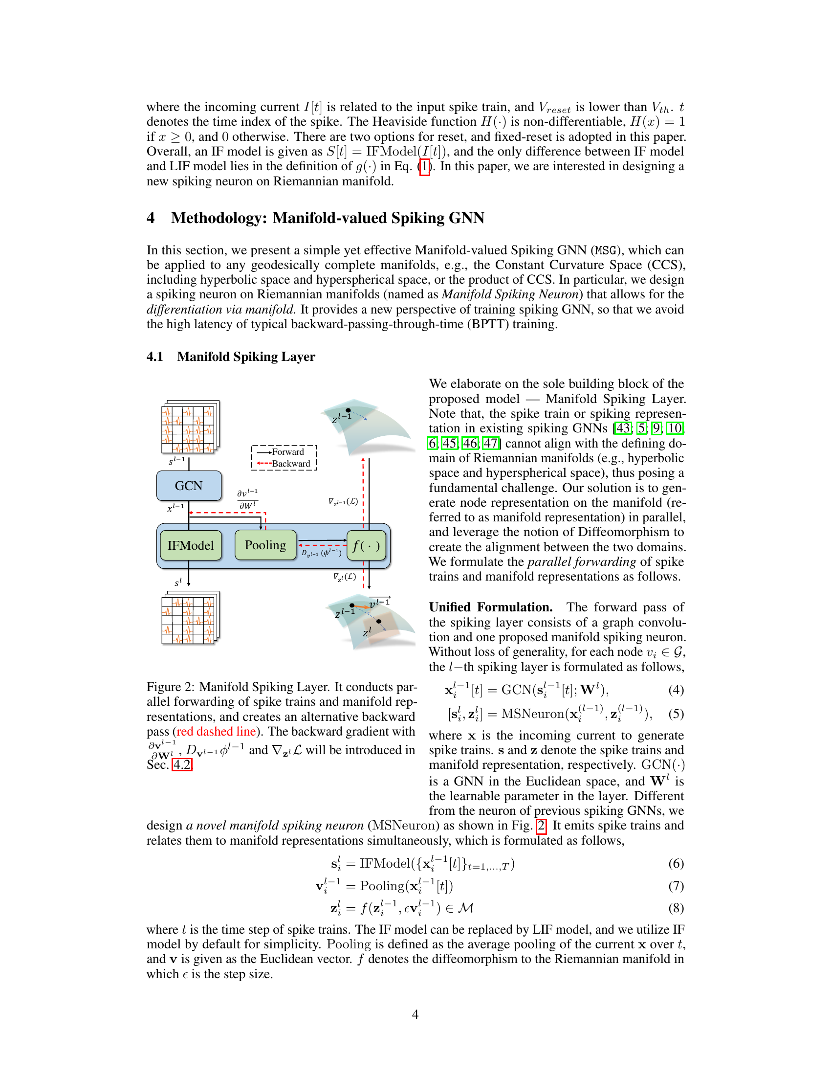
🔼 This figure illustrates the architecture of a Manifold Spiking Layer, a key component of the proposed Manifold-valued Spiking GNN (MSG). It shows how the layer processes both spike trains (representing temporal information) and manifold representations (representing spatial/structural information) in parallel. The forward pass involves graph convolution (GCN) and a manifold spiking neuron (MSNeuron). The backward pass, however, deviates from standard backpropagation through time (BPTT) by employing a novel method called Differentiation via Manifold (DvM), represented by the red dashed line. This DvM method is designed to improve efficiency and overcome latency issues associated with BPTT in spiking neural networks.
read the caption
Figure 2: Manifold Spiking Layer. It conducts parallel forwarding of spike trains and manifold representations, and creates an alternative backward pass (red dashed line). The backward gradient with w, Dl-1-1-1 and ∇zl L will be introduced in Sec. 4.2.

🔼 This figure illustrates the concept of charts in the context of Riemannian manifolds. A chart is a local mapping between a region of the manifold and a Euclidean space. In this image, we see three charts (U₁, φ₁), (U₂, φ₂), and (U₃, φ₃), each covering a different part of a curved, two-dimensional manifold. The logarithmic map is used to create these charts, mapping points on the manifold to corresponding points in tangent spaces that are locally Euclidean. The figure shows the process of using a series of charts to approximate a continuous path (the red dotted line) on the manifold, which is a common technique in solving manifold ordinary differential equations (ODEs). This visual helps explain the theoretical foundation of how the proposed model approximates a dynamic chart solver for manifold ODEs.
read the caption
Figure 3: Charts given by the logarithmic map.

🔼 This figure illustrates the architecture of the Manifold Spiking Layer, a key component of the proposed Manifold-valued Spiking GNN (MSG). It shows how the layer performs parallel processing of spike trains (representing information from spiking neurons) and manifold representations (representing data on a Riemannian manifold). The diagram highlights the novel backward pass mechanism (represented by the red dashed line) that replaces the traditional Back-Propagation-Through-Time (BPTT) method with the proposed Differentiation via Manifold (DvM) for efficient training. The backward gradient calculation involves terms ‘w’, ‘Dl−1zl−1’, and ‘∇zlL’, which are detailed in section 4.2 of the paper.
read the caption
Figure 2: Manifold Spiking Layer. It conducts parallel forwarding of spike trains and manifold representations, and creates an alternative backward pass (red dashed line). The backward gradient with w, Dl−1zl−1 and ∇zlL will be introduced in Sec. 4.2.

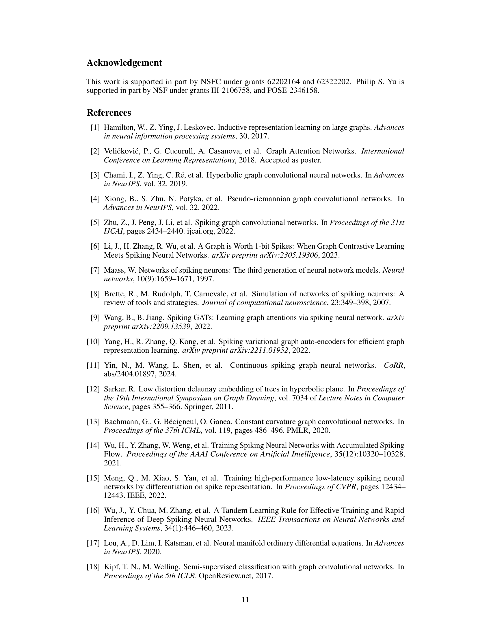
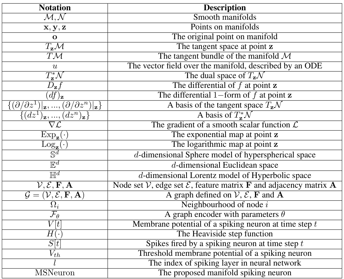
🔼 This figure visualizes the proposed model’s behavior on a torus (S¹ × S¹). Each point represents a node’s representation at a specific layer in the model. The red curve shows the path of a node’s representation across layers, illustrating how it evolves through the manifold. The blue arrows indicate the direction of the geodesic (the shortest path) along which the node’s representation moves within the manifold at each layer. This demonstrates how the model iteratively solves an ODE on the manifold, effectively navigating the complex geometric structure of the graph.
read the caption
Figure 5: Visualization on S¹ × S¹.

🔼 This figure visualizes the training process of the proposed model using the Differentiation via Manifold (DvM) method. It shows the norm of backward gradients for each layer and the overall loss during training. The results demonstrate the effectiveness of DvM, which avoids gradient vanishing or explosion.
read the caption
Figure 6: Visualizations of the training process for node classification on Computer dataset. Backward Gradient. Previous studies compute backward gradients though the Differentiation via Spikes (DvS). Distinguishing from the previous studies, we compute backward gradients though the Differentiation via Manifold (DvM). In order to examine the backward gradients, we visualize the training process for node classification on Computer dataset. Concretely, we plot the norm of backward gradients in each iteration in Figs. 6 (a) and (b) together with the value of loss function in Figs. 6 (c). As shown in Fig. 6, the proposed algorithm with DvM converges well, and the backward gradients do not suffer from gradient vanishing or gradient explosion.

🔼 This figure visualizes the training process of the proposed model (MSG) on the Computer dataset. It compares the backward gradient norms using Differentiation via Spikes (DvS) and the proposed Differentiation via Manifold (DvM). The plots show the norm of backward gradients with respect to z and v in each layer, as well as the overall training loss. The results demonstrate that the proposed DvM method effectively avoids gradient vanishing and explosion, leading to faster convergence.
read the caption
Figure 6: Visualizations of the training process for node classification on Computer dataset. Backward Gradient. Previous studies compute backward gradients though the Differentiation via Spikes (DvS). Distinguishing from the previous studies, we compute backward gradients though the Differentiation via Manifold (DvM). In order to examine the backward gradients, we visualize the training process for node classification on Computer dataset. Concretely, we plot the norm of backward gradients in each iteration in Figs. 6 (a) and (b) together with the value of loss function in Figs. 6 (c). As shown in Fig. 6, the proposed algorithm with DvM converges well, and the backward gradients do not suffer from gradient vanishing or gradient explosion.

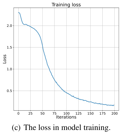
🔼 This figure visualizes the training process of the proposed model (MSG) on the Computer dataset. It shows the norm of backward gradients for both z and v in each layer, along with the training loss. This demonstrates the effectiveness of the proposed Differentiation via Manifold (DvM) method, highlighting its convergence and lack of gradient vanishing/explosion compared to the traditional Differentiation via Spikes (DvS).
read the caption
Figure 6: Visualizations of the training process for node classification on Computer dataset. Backward Gradient. Previous studies compute backward gradients though the Differentiation via Spikes (DvS). Distinguishing from the previous studies, we compute backward gradients though the Differentiation via Manifold (DvM). In order to examine the backward gradients, we visualize the training process for node classification on Computer dataset. Concretely, we plot the norm of backward gradients in each iteration in Figs. 6 (a) and (b) together with the value of loss function in Figs. 6 (c). As shown in Fig. 6, the proposed algorithm with DvM converges well, and the backward gradients do not suffer from gradient vanishing or gradient explosion.

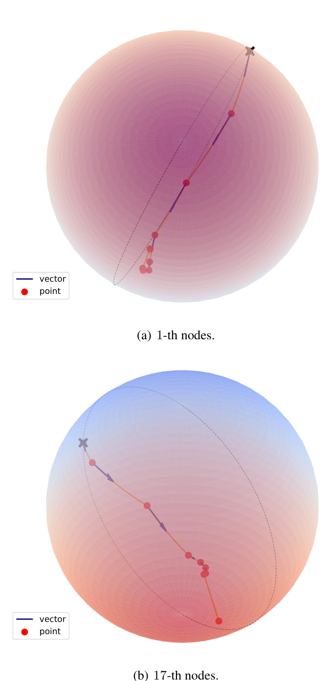
🔼 This figure visualizes node representations on the Zachary Karate Club dataset using the proposed Manifold-valued Spiking GNN (MSG). It shows the node representations at each spiking layer for two specific nodes (1-th and 17-th). The red dots represent the manifold representation of the node at each layer, while the blue lines represent the tangent vectors (directions) that guide the movement of the node representations along geodesics on the manifold. The curves connecting the outputs of successive layers are marked in red, illustrating how each layer’s computation contributes to the overall progression. This visualization empirically demonstrates the relationship between MSG and manifold ordinary differential equations (ODEs), as each layer acts as a solver of the ODE describing the geodesic on the manifold.
read the caption
Figure 7: Visualizations of node representations on Zachary karateClub datasets [58].

More on tables

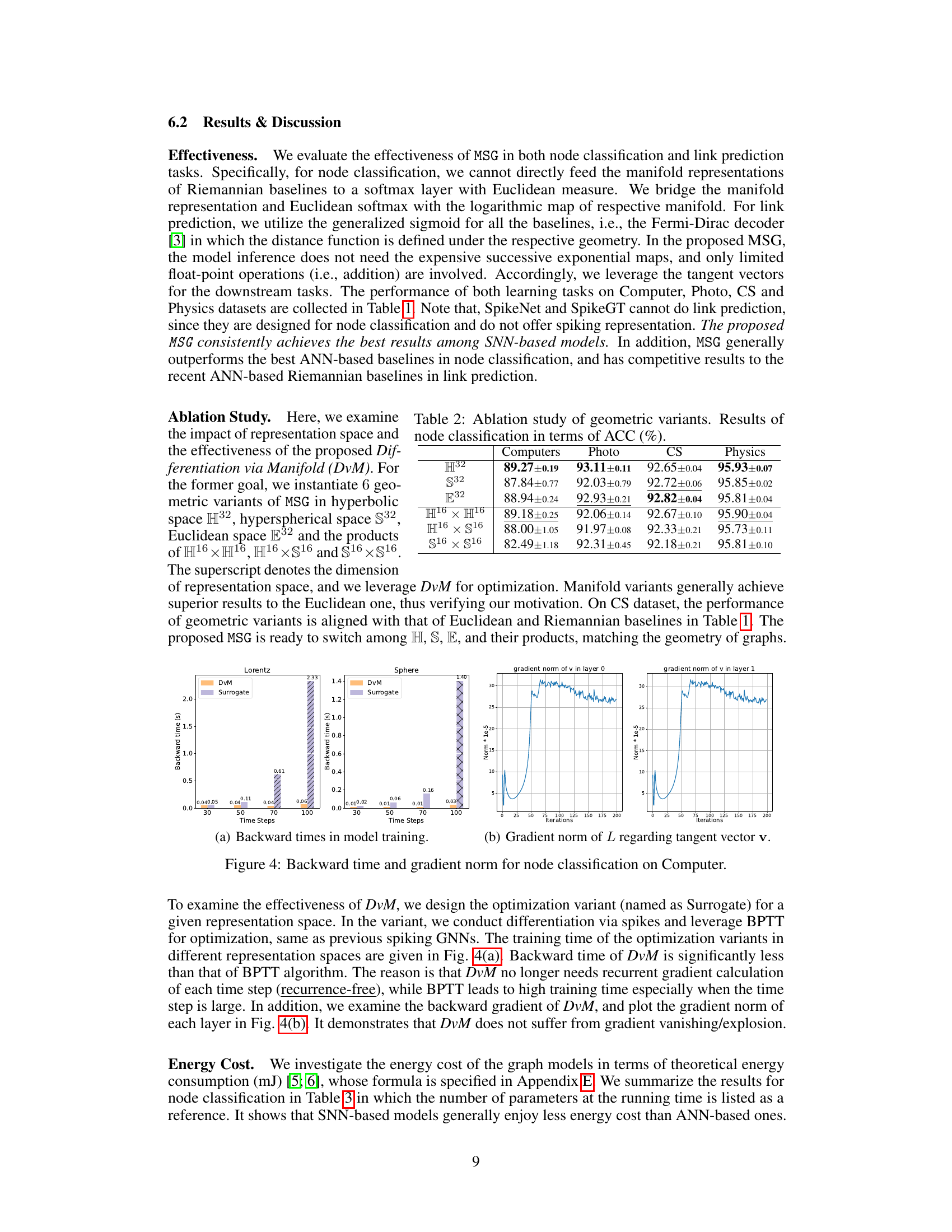
🔼 This table presents the results of an ablation study comparing different geometric variants of the proposed Manifold-valued Spiking GNN (MSG) model. The variants use different types of Riemannian manifolds for representation (hyperbolic H³², hyperspherical S³², Euclidean E³², and products of these spaces). Node classification accuracy (ACC) is reported for each variant across four datasets (Computers, Photo, CS, Physics). The purpose is to demonstrate the impact of the choice of manifold on model performance.
read the caption
Table 2: Ablation study of geometric variants. Results of node classification in terms of ACC (%).

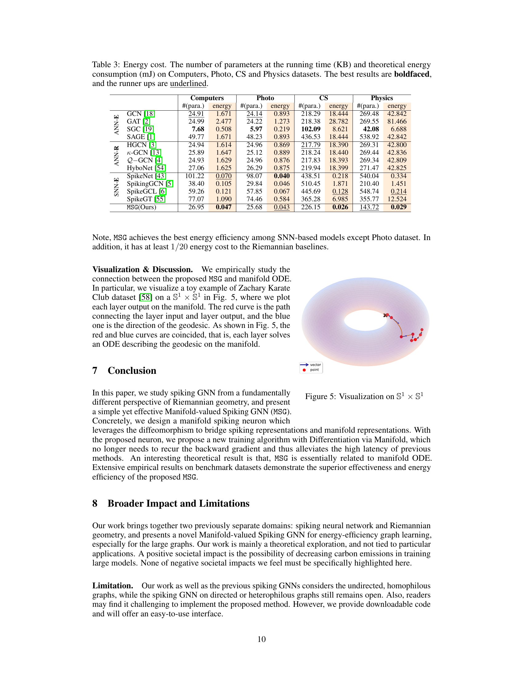
🔼 This table presents a comparison of energy costs and parameter counts for various graph neural network models (both ANN-based and SNN-based) across four benchmark datasets. The energy consumption is theoretically calculated, not measured empirically. The table highlights the superior energy efficiency of spiking neural networks (SNNs) compared to artificial neural networks (ANNs), particularly the proposed MSG model.
read the caption
Table 3: Energy cost, the number of parameters at the running time (KB) and theoretical energy consumption (mJ) on Computers, Photo, CS and Physics datasets. The best results are boldfaced, and the runner ups are underlined.

🔼 This table presents a comparison of different graph neural network models’ performance on four benchmark datasets (Computers, Photo, CS, and Physics). The performance is evaluated using two metrics: node classification accuracy and link prediction AUC. The table includes both ANN-based (Euclidean and Riemannian) and SNN-based (Euclidean) models, highlighting the superior performance of the proposed MSG model (boldfaced). The inclusion of both ANN and SNN models allows for a direct comparison of the effectiveness and efficiency of different approaches.
read the caption
Table 1: Node Classification (NC) in terms of classification accuracy (%) and Link Prediction in terms of AUC (%) on Computers, Photo, CS and Physics datasets. The best results are boldfaced, and the runner-ups are underlined.

🔼 This table presents the performance comparison of node classification accuracy and link prediction AUC on four benchmark datasets (Computers, Photo, CS, Physics) using different graph neural network (GNN) models. It compares both ANN-based (Euclidean and Riemannian) and SNN-based (Euclidean) methods, highlighting the proposed MSG’s performance against the existing state-of-the-art models.
read the caption
Table 1: Node Classification (NC) in terms of classification accuracy (%) and Link Prediction in terms of AUC (%) on Computers, Photo, CS and Physics datasets. The best results are boldfaced, and the runner-ups are underlined. The standard derivations are given in the subscripts.

🔼 This table compares the performance of the proposed MSG model against 12 other baseline models on four benchmark datasets (Computers, Photo, CS, Physics) for two graph learning tasks: node classification and link prediction. The results are presented as classification accuracy (%) and AUC (%). The best performing model for each dataset and task is shown in bold, and the second-best is underlined. The table highlights the superior performance of the proposed MSG model, especially in terms of node classification.
read the caption
Table 1: Node Classification (NC) in terms of classification accuracy (%) and Link Prediction in terms of AUC (%) on Computers, Photo, CS and Physics datasets. The best results are boldfaced, and the runner-ups are underlined.

🔼 This table compares the performance of the proposed Manifold-valued Spiking GNN (MSG) model using two different spiking neuron models: Integrate-and-Fire (IF) and Leaky Integrate-and-Fire (LIF). The comparison is done across four different datasets (Computers, Photo, CS, Physics) and three different geometric manifold types (hyperbolic H³², hyperspherical S³², Euclidean E³²). The training method used is Differentiation via Spikes (DvS), which leverages Backpropagation Through Time (BPTT) with a surrogate gradient. The table shows the classification accuracy (%) for each combination of neuron model, dataset, and manifold type.
read the caption
Table 7: Comparison between IF and LIF model in Node Classification, qualified by classification accuracy (%). The proposed model is trained by Differentiation via Spikes (i.e., BPTT with the surrogate gradient).

🔼 This table presents the results of node classification and link prediction experiments on four benchmark datasets (Computers, Photo, CS, Physics). It compares the performance of the proposed Manifold-valued Spiking GNN (MSG) against twelve other methods, including both traditional ANN-based GNNs (on Euclidean and Riemannian manifolds) and previous spiking GNNs (on Euclidean manifolds only). The best performance for each dataset and task is shown in bold, with second-best results underlined. The results highlight MSG’s superior performance.
read the caption
Table 1: Node Classification (NC) in terms of classification accuracy (%) and Link Prediction in terms of AUC (%) on Computers, Photo, CS and Physics datasets. The best results are boldfaced, and the runner-ups are underlined.

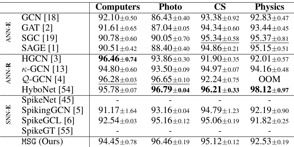
🔼 This table presents a comparison of various graph neural network models (both ANN-based and SNN-based) on four benchmark datasets (Computers, Photo, CS, Physics). The performance is evaluated using two metrics: Node Classification accuracy and Link Prediction AUC. The best performing model for each dataset and metric is highlighted in bold, with the second-best underlined. Standard deviations are also included to show the variability of the results.
read the caption
Table 1: Node Classification (NC) in terms of classification accuracy (%) and Link Prediction in terms of AUC (%) on Computers, Photo, CS and Physics datasets. The best results are boldfaced, and the runner-ups are underlined. The standard derivations are given in the subscripts.

TL;DR#

Key Takeaways#

Why does it matter?#

Visual Insights#

In-depth insights#

Riemannian SNNs#

Manifold Spiking#

DvM Training#

MSG Neural ODE#

Future Works#

More visual insights#

Full paper#