TL;DR#
Many machine learning models fail when encountering data that differs significantly from their training data (out-of-distribution or OOD). Existing methods for OOD detection often struggle to reliably identify such outliers, especially those near the decision boundary between in-distribution and out-of-distribution data. This is particularly problematic when deploying these models in real-world scenarios where unexpected data is common. This necessitates more robust and accurate OOD detection techniques.
This paper introduces Hopfield Boosting, a novel method that addresses these challenges. Hopfield Boosting uses an energy-based approach that leverages modern Hopfield networks to better define the decision boundary, improving accuracy. The method also incorporates an auxiliary outlier dataset to further enhance its capability of detecting hard-to-classify outliers that are close to the decision boundary. Experimental results demonstrate that Hopfield Boosting achieves state-of-the-art performance on several benchmark datasets, showing marked improvements over existing approaches.
Key Takeaways#
Why does it matter?#
This paper is crucial for researchers working on out-of-distribution (OOD) detection, a critical challenge in real-world machine learning deployments. It introduces a novel boosting method that significantly improves OOD detection performance. The Hopfield Boosting approach and its theoretical backing provide new avenues for research, particularly in the use of energy-based models and the strategic sampling of training data. This will likely influence future work in OOD detection and related areas.
Visual Insights#
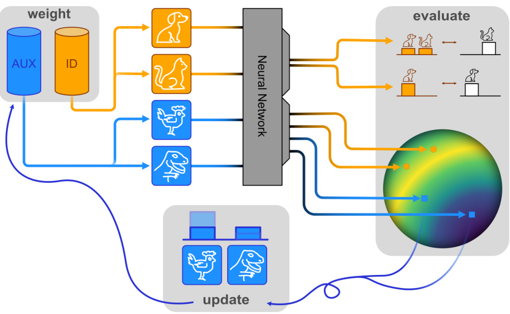
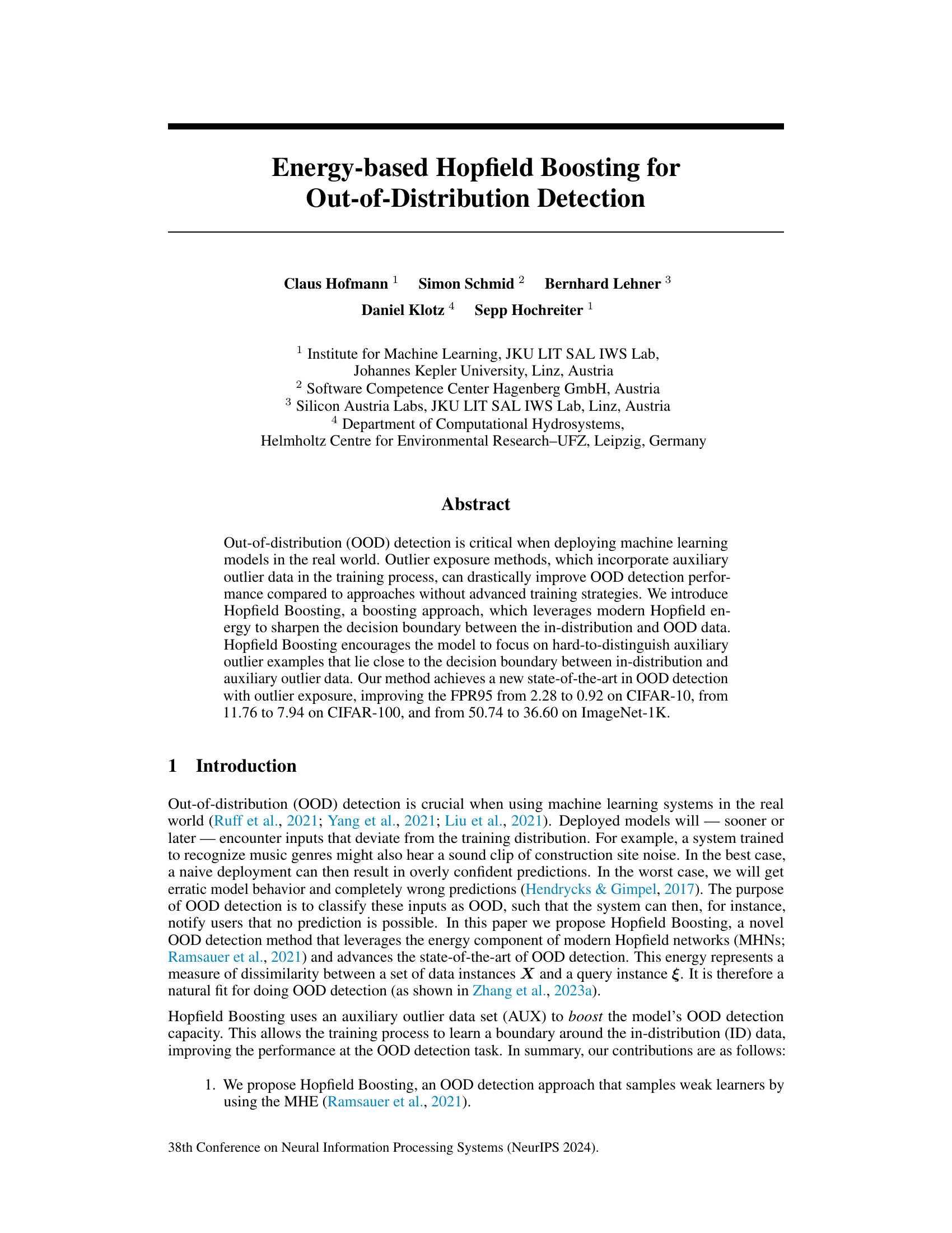
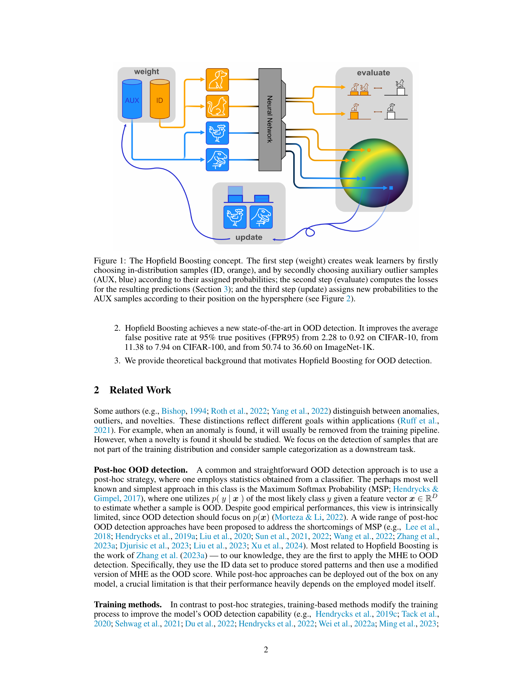
🔼 This figure illustrates the Hopfield Boosting concept, showing a three-step process. First, weak learners are created by sampling in-distribution (ID) and auxiliary outlier (AUX) data based on their assigned probabilities. Second, the model evaluates the performance of these learners by computing losses on the resulting predictions. Finally, the model updates the probabilities for the AUX samples based on their position on a hypersphere, guiding the focus on challenging outlier samples near the decision boundary.
read the caption
Figure 1: The Hopfield Boosting concept. The first step (weight) creates weak learners by firstly choosing in-distribution samples (ID, orange), and by secondly choosing auxiliary outlier samples (AUX, blue) according to their assigned probabilities; the second step (evaluate) computes the losses for the resulting predictions (Section 3); and the third step (update) assigns new probabilities to the AUX samples according to their position on the hypersphere (see Figure 2).

🔼 This table presents a comparison of the out-of-distribution (OOD) detection performance of Hopfield Boosting against several state-of-the-art methods on the CIFAR-10 dataset. Metrics used include the false positive rate at 95% true positives (FPR95) and the area under the receiver operating characteristic curve (AUROC). Lower FPR95 and higher AUROC values indicate better performance. Results are shown for different OOD datasets and include standard deviations calculated from five training runs.
read the caption
Table 1: OOD detection performance on CIFAR-10. We compare results from Hopfield Boosting, DOS (Jiang et al., 2024), DOE (Wang et al., 2023b), DivOE (Zhu et al., 2023), DAL (Wang et al., 2023a), MixOE (Zhang et al., 2023b), POEM (Ming et al., 2022), EBO-OE (Liu et al., 2020), and MSP-OE (Hendrycks et al., 2019b) on ResNet-18. ↓ indicates “lower is better” and ↑ “higher is better”. All values in %. Standard deviations are estimated across five training runs.
In-depth insights#
Hopfield Boosting#
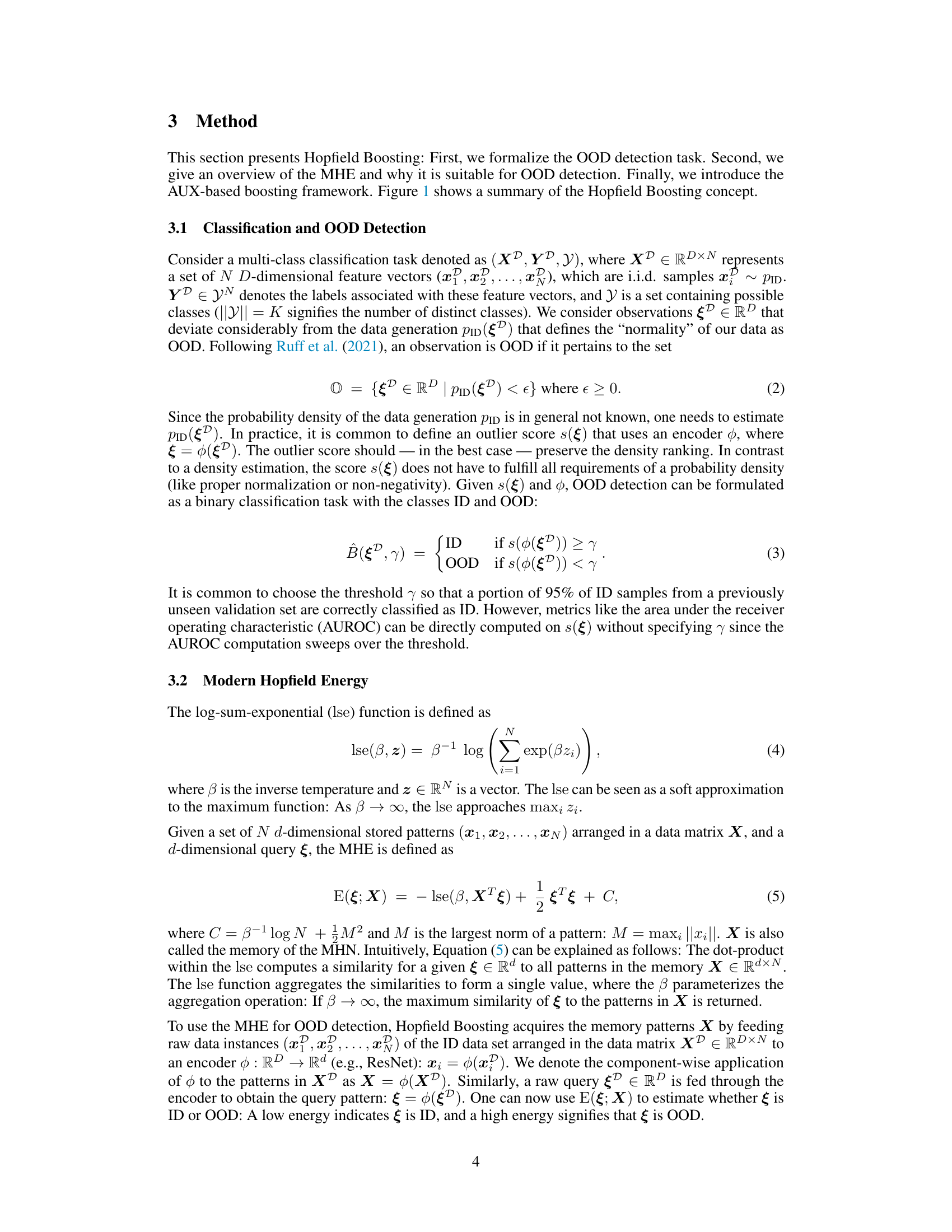
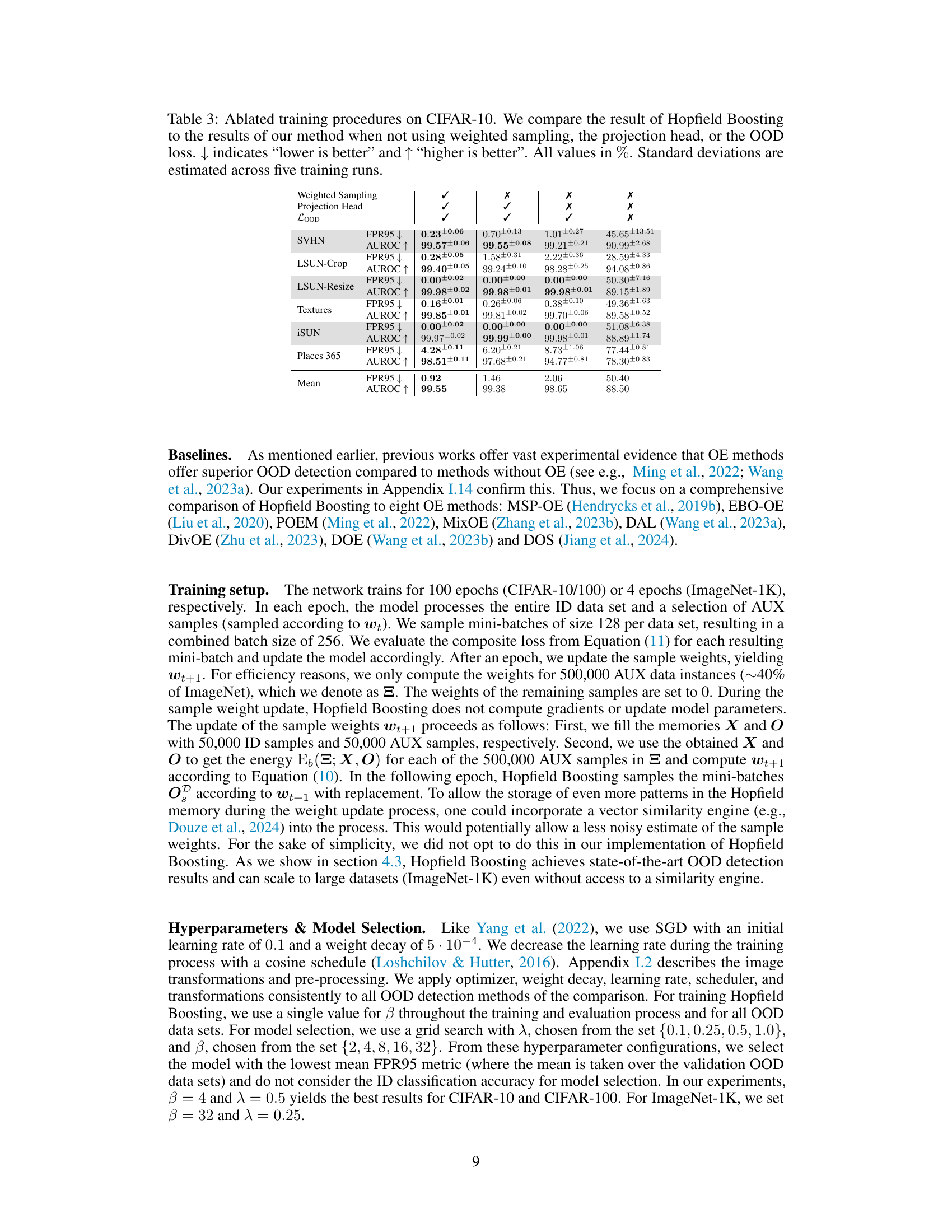
Hopfield Boosting, as presented in the research paper, is a novel boosting approach for out-of-distribution (OOD) detection that leverages the energy function of modern Hopfield networks. The core idea is to sharpen the decision boundary between in-distribution and OOD data by focusing on the most challenging outlier examples close to the decision boundary. This is achieved by sampling weak learners (both in-distribution and auxiliary outlier samples) based on their probabilities, which are updated iteratively in a boosting-like fashion. This adaptive resampling approach helps the model prioritize those data instances that are hard to distinguish, effectively improving the model’s OOD detection performance. Hopfield Boosting enhances the existing outlier exposure (OE) methods by using a more informative sample selection strategy. In addition to the empirical results showing a significant improvement on several benchmark datasets, the paper provides a theoretical foundation, demonstrating that Hopfield Boosting is related to well-known techniques like radial basis function networks and support vector machines, lending further credibility to its effectiveness. The theoretical analysis also helps to explain how the method effectively leverages the energy function to improve its discrimination between the in-distribution and the outliers. Hopfield Boosting’s success is mainly attributed to its adaptive sampling and sophisticated energy-based training which allows for a tighter decision boundary and better generalization to previously unseen OOD data.
OOD Detection#
Out-of-distribution (OOD) detection is crucial for deploying machine learning models reliably in real-world scenarios. The core challenge lies in a model’s ability to discern between data points originating from its training distribution (in-distribution) and those that don’t (out-of-distribution). Common approaches involve post-hoc methods, which analyze model outputs to assign an OOD score, and training-based methods, which incorporate auxiliary outlier data during training to improve the model’s ability to recognize outliers. Hopfield Boosting, as presented in the paper, offers a novel training-based method. It leverages the energy component of modern Hopfield networks to sharpen the decision boundary between in-distribution and out-of-distribution data. The method focuses on the ‘hard’ to distinguish outliers close to the decision boundary for improved learning. Hopfield Boosting is shown to improve upon previous state-of-the-art methods, achieving significant gains in OOD detection performance across various benchmark datasets. However, challenges remain, as the paper identifies limitations in the reliability of OOD detection across datasets with specific characteristics and the potential for misinterpretation of OOD scores. Future research should explore these limitations and further refine OOD detection techniques.
Energy-Based#
The concept of ‘Energy-Based’ in the context of machine learning, particularly within the framework of out-of-distribution (OOD) detection, offers a compelling approach. It leverages the principles of energy-based models, where the energy function quantifies the compatibility of an input with the learned distribution. Lower energy indicates a data point belonging to the in-distribution, while higher energy signals an outlier or OOD sample. This provides an intuitive and elegant way to differentiate between normal and anomalous data. This approach contrasts with other methods, and the energy-based approach may offer advantages in terms of interpretability and robustness, enabling the model to focus on inherently difficult-to-classify samples near the decision boundary. This ‘Energy-Based’ method is particularly useful when dealing with complex data distributions or imbalanced datasets. The Hopfield network, with its energy-based architecture, appears as a suitable candidate for implementing such an approach. The energy function in a Hopfield network naturally lends itself to OOD detection tasks, providing a principled way to assess the degree of dissimilarity between an input and the known in-distribution patterns. Therefore, combining energy-based methods and Hopfield networks offers a promising direction for advancing OOD detection.
OE Methods#
Outlier Exposure (OE) methods represent a significant advancement in out-of-distribution (OOD) detection. OE’s core principle is to augment training data with auxiliary outlier data, forcing the model to learn a more robust decision boundary that effectively separates in-distribution (ID) from OOD samples. This contrasts sharply with traditional methods, which often struggle with OOD samples due to a lack of exposure during training. The effectiveness of OE methods hinges on several crucial factors. First, the selection of auxiliary data is paramount. Carefully chosen outliers that lie close to the decision boundary are most effective in refining model performance. Second, the method of integrating auxiliary data matters. Simply adding outliers might not be sufficient; techniques like Hopfield Boosting, discussed in the paper, employ sophisticated strategies such as weighted sampling to focus on the most informative outliers. Third, the choice of loss function plays a critical role. Effective loss functions should incentivize the model to learn a sharp boundary, penalizing uncertainty in areas near the decision boundary. In conclusion, OE methods represent a powerful paradigm shift in OOD detection, offering substantial improvements over traditional techniques when properly implemented. However, challenges remain in selecting optimal auxiliary datasets and designing efficient integration strategies; future research should address these aspects to fully unleash the potential of OE methods.
Future Work#
The ‘Future Work’ section of a research paper on Hopfield Boosting for out-of-distribution detection offers exciting avenues for improvement and expansion. One key area is a deeper investigation into the nature of the decision boundary shaped by the method. Analyzing how the boundary’s smoothness and sharpness affect model performance, particularly in the context of adversarial examples and robustness, would be significant. The authors suggest exploring the impact of the ‘sharpening’ effect on adversarial robustness, proposing it as a potential area of future research. This would involve a systematic comparison between models trained with and without this ‘sharpening’ method, using various adversarial attacks. Another important consideration is developing a more comprehensive and robust metric for evaluating OOD detection methods. The current metrics, while useful, don’t fully capture the nuances of real-world OOD scenarios. Investigating alternative metrics and combining existing ones might lead to more accurate and nuanced evaluations. Finally, scaling Hopfield Boosting to handle very large datasets efficiently is crucial for real-world applications. This involves exploring optimization techniques and potentially integrating approximate nearest neighbor search methods. Addressing these aspects of future work will enhance the practical applicability and impact of Hopfield Boosting for OOD detection.
More visual insights#
More on figures

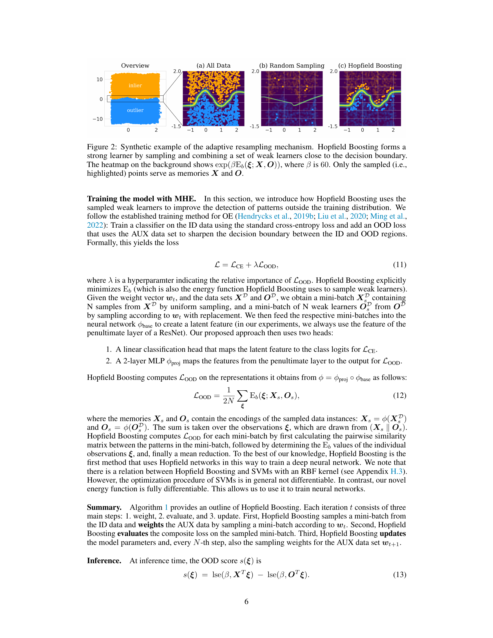
🔼 This figure shows a synthetic example to illustrate the adaptive resampling mechanism in Hopfield Boosting. It compares three scenarios: using all data, random sampling, and Hopfield Boosting’s adaptive sampling. Hopfield Boosting focuses on selecting weak learners near the decision boundary, resulting in a stronger ensemble learner and a tighter decision boundary (shown by the heatmap representing the exponentiated Hopfield energy).
read the caption
Figure 2: Synthetic example of the adaptive resampling mechanism. Hopfield Boosting forms a strong learner by sampling and combining a set of weak learners close to the decision boundary. The heatmap on the background shows exp(βE♭(ξ; X, O)), where β is 60. Only the sampled (i.e., highlighted) points serve as memories X and O.
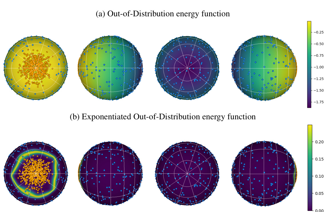
🔼 This figure shows the energy function E♭(ξ; X, O) represented on a 3D hypersphere. The energy function is used to sample weak learners in the Hopfield Boosting algorithm. Part (a) shows the energy function itself; Part (b) shows the exponential of the energy function, which highlights the areas of high energy more clearly. The plots are rotated to show the function from different perspectives.
read the caption
Figure 3: Depiction of the energy function E♭(ξ; X, O) on a hypersphere. (a) shows E♭(ξ, Χ, Ο) with exemplary inlier (orange) and outlier (blue) points; and (b) shows exp(βE♭(ξ, Χ, Ο)). β was set to 128. Both, (a) and (b), rotate the sphere by 0, 90, 180, and 270 degrees around the vertical axis.
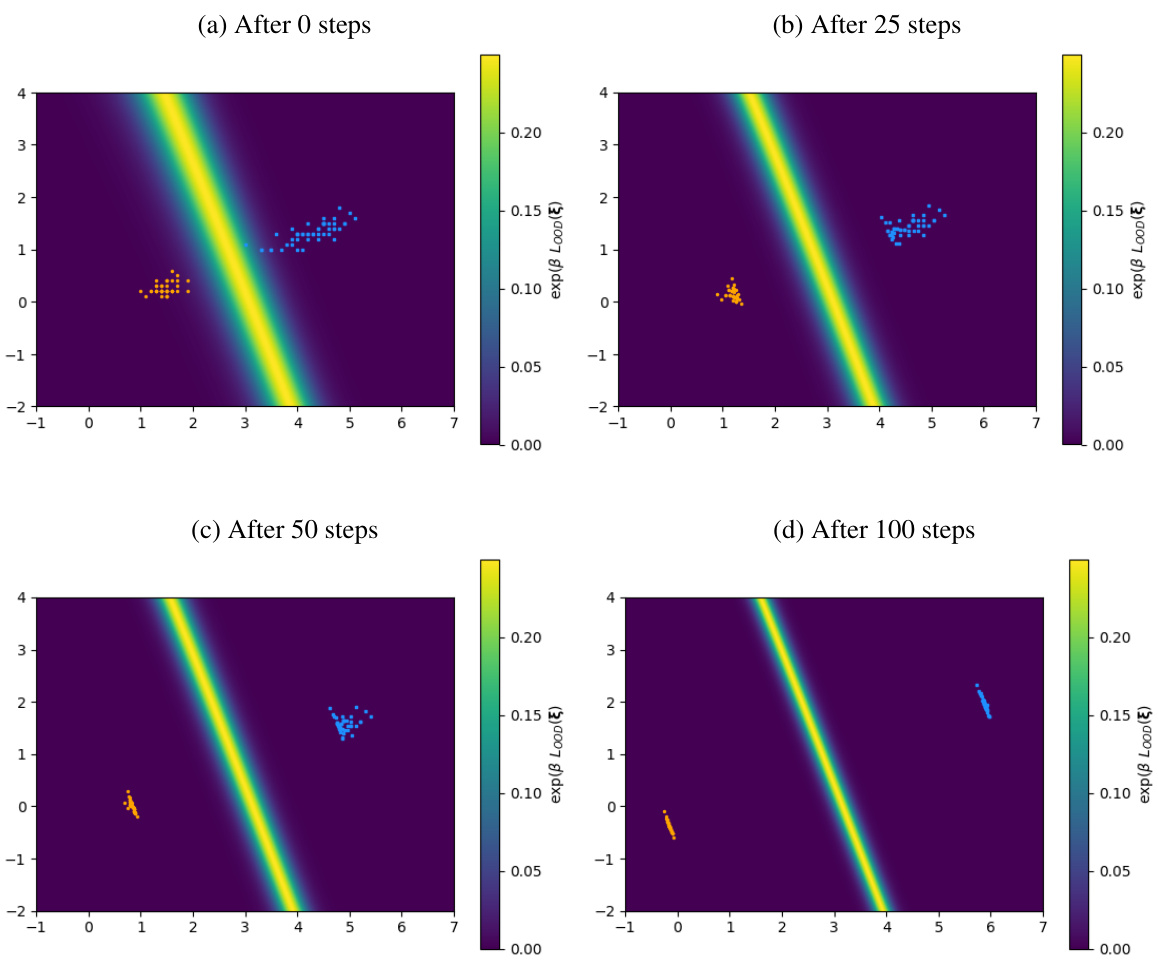
🔼 This figure shows how Hopfield Boosting adaptively resamples weak learners near the decision boundary. The heatmap represents the energy function, with higher values indicating points closer to the boundary. The orange points represent in-distribution samples, while the blue points are auxiliary outliers. By focusing on these hard-to-classify samples, Hopfield Boosting improves the model’s ability to distinguish between in-distribution and out-of-distribution data.
read the caption
Figure 2: Synthetic example of the adaptive resampling mechanism. Hopfield Boosting forms a strong learner by sampling and combining a set of weak learners close to the decision boundary. The heatmap on the background shows exp(βE♭(ξ; X, O)), where β is 60. Only the sampled (i.e., highlighted) points serve as memories X and O.
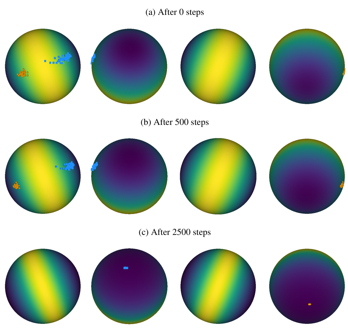
🔼 The figure shows how the energy-based loss function shapes the decision boundary between in-distribution and out-of-distribution data. The energy landscape is visualized on a 3D hypersphere. In-distribution points (orange) cluster around one pole, while out-of-distribution points (blue) are distributed across the rest of the sphere. The gradient descent updates push the outliers toward the opposite pole from the inliers, creating a clear separation between the two classes.
read the caption
Figure 5: LOOD applied to exemplary data points on a sphere. Gradients are applied to the data points directly. We observe that the geometry of the space forces the patterns to opposing poles of the sphere.
🔼 This figure shows how Hopfield Boosting adaptively resamples data points near the decision boundary to create a strong learner by combining many weak learners. The heatmap visualizes the energy function, showing high energy (darker colors) further from the boundary and low energy (lighter colors) near the boundary. Only the sampled points contribute to the strong learner.
read the caption
Figure 2: Synthetic example of the adaptive resampling mechanism. Hopfield Boosting forms a strong learner by sampling and combining a set of weak learners close to the decision boundary. The heatmap on the background shows exp(βE♭(ξ; X, O)), where β is 60. Only the sampled (i.e., highlighted) points serve as memories X and O.

🔼 This figure shows a 3D visualization of the energy function Eb on a hypersphere, demonstrating how inliers and outliers shape the energy surface. It’s shown in two variations: (a) shows Eb itself, and (b) shows the exponentiation of Eb, which accentuates the differences in energy levels. The visualization is presented from four different angles (0, 90, 180, and 270 degrees rotation around the vertical axis).
read the caption
Figure 3: Depiction of the energy function Eb(ξ; X, O) on a hypersphere. (a) shows Eb(ξ, X, O) with exemplary inlier (orange) and outlier (blue) points; and (b) shows exp(βEb(ξ, X, O)). β was set to 128. Both, (a) and (b), rotate the sphere by 0, 90, 180, and 270 degrees around the vertical axis.

🔼 This figure demonstrates the adaptive resampling mechanism of Hopfield Boosting. It shows how Hopfield Boosting forms a strong learner by sampling and combining weak learners that are close to the decision boundary. The heatmap visualizes the energy function, highlighting the area where the weak learners are sampled. Only the selected points (highlighted) serve as memories in the Hopfield network.
read the caption
Figure 2: Synthetic example of the adaptive resampling mechanism. Hopfield Boosting forms a strong learner by sampling and combining a set of weak learners close to the decision boundary. The heatmap on the background shows exp(βE♭(ξ; X, O)), where β is 60. Only the sampled (i.e., highlighted) points serve as memories X and O.

🔼 This figure shows the energy function E♭(ξ; X, O) and its exponential form on a 3D hypersphere. The orange and blue points represent inliers and outliers, respectively. The plots visualize how the energy landscape changes based on the positioning of inliers and outliers, illustrating the model’s ability to separate in-distribution (ID) and out-of-distribution (OOD) data using the Hopfield energy.
read the caption
Figure 3: Depiction of the energy function E♭(ξ; X, O) on a hypersphere. (a) shows E♭(ξ, Χ, Ο) with exemplary inlier (orange) and outlier (blue) points; and (b) shows exp(βE♭(ξ, Χ, Ο)). β was set to 128. Both, (a) and (b), rotate the sphere by 0, 90, 180, and 270 degrees around the vertical axis.

🔼 This figure shows how Hopfield Boosting adaptively resamples weak learners near the decision boundary between in-distribution (ID) and out-of-distribution (OOD) data. By focusing on these hard-to-distinguish samples, it creates a strong learner that effectively separates ID and OOD data. The background heatmap visualizes the energy function, with darker colors indicating higher energy (and thus, weaker learners).
read the caption
Figure 2: Synthetic example of the adaptive resampling mechanism. Hopfield Boosting forms a strong learner by sampling and combining a set of weak learners close to the decision boundary. The heatmap on the background shows exp(βE♭(ξ; X, O)), where β is 60. Only the sampled (i.e., highlighted) points serve as memories X and O.
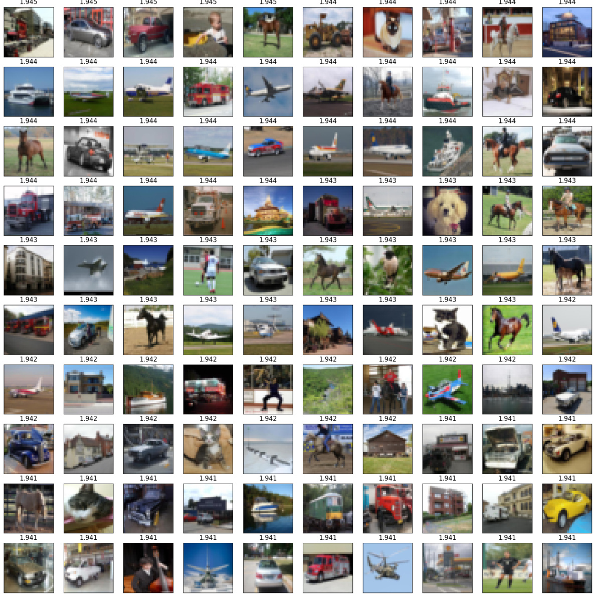
🔼 This figure demonstrates how Hopfield Boosting adaptively resamples weak learners near the decision boundary to create a strong learner. The leftmost panel shows all data points, with inliers (orange) and outliers (blue) clearly separated. The middle panel demonstrates random sampling, while the rightmost panel showcases Hopfield Boosting’s selective sampling strategy, focusing on the boundary region. A heatmap in the background represents the energy function, illustrating the concentration of sampled points (highlighted) near the decision boundary.
read the caption
Figure 2: Synthetic example of the adaptive resampling mechanism. Hopfield Boosting forms a strong learner by sampling and combining a set of weak learners close to the decision boundary. The heatmap on the background shows exp(βE♭(ξ; X, O)), where β is 60. Only the sampled (i.e., highlighted) points serve as memories X and O.
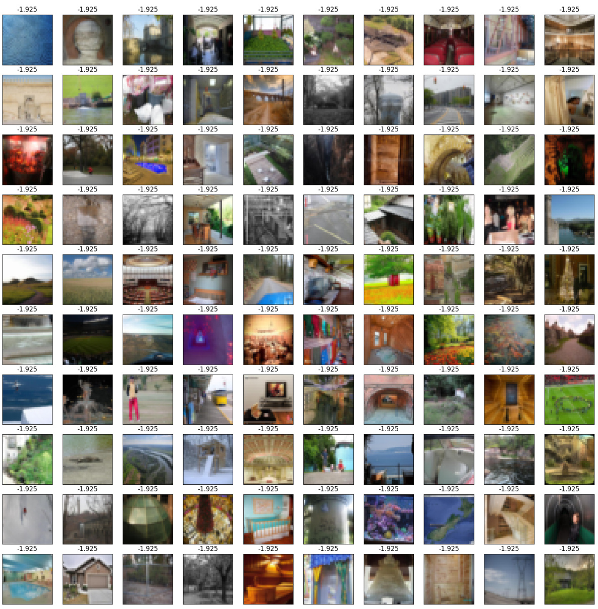
🔼 This figure demonstrates how Hopfield Boosting adaptively resamples data points near the decision boundary. The heatmap shows the energy function (exp(βE♭(ξ; X, O))), with darker colors indicating higher energy and thus, points closer to the boundary between in-distribution and outlier data. Hopfield Boosting emphasizes these ‘hard-to-classify’ points (the highlighted points) as weak learners and combines them to form a strong learner, thereby improving the accuracy of the decision boundary. The sampling is not random; rather, it’s weighted, focusing on weak learners that improve OOD detection.
read the caption
Figure 2: Synthetic example of the adaptive resampling mechanism. Hopfield Boosting forms a strong learner by sampling and combining a set of weak learners close to the decision boundary. The heatmap on the background shows exp(βE♭(ξ; X, O)), where β is 60. Only the sampled (i.e., highlighted) points serve as memories X and O.

🔼 This figure illustrates the Hopfield Boosting concept, which is a three-step process. In the first step, weak learners are created by sampling in-distribution (ID) and auxiliary outlier (AUX) samples based on their probabilities. The second step evaluates the losses for the predictions made by these weak learners. Finally, the third step updates the probabilities of the AUX samples based on their position on a hypersphere, effectively focusing on the hard-to-distinguish samples near the decision boundary.
read the caption
Figure 1: The Hopfield Boosting concept. The first step (weight) creates weak learners by firstly choosing in-distribution samples (ID, orange), and by secondly choosing auxiliary outlier samples (AUX, blue) according to their assigned probabilities; the second step (evaluate) computes the losses for the resulting predictions (Section 3); and the third step (update) assigns new probabilities to the AUX samples according to their position on the hypersphere (see Figure 2).
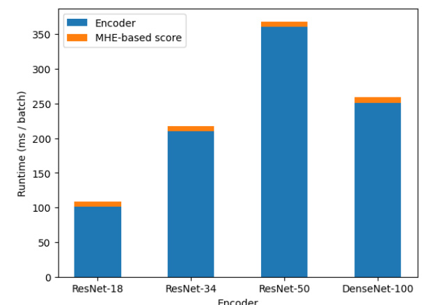
🔼 This figure shows a synthetic example to illustrate how Hopfield Boosting adaptively resamples data points near the decision boundary. The leftmost panel shows all the data points; the middle panel shows random sampling; the rightmost panel shows Hopfield Boosting’s approach. Hopfield Boosting’s resampling strategy focuses on samples near the decision boundary, which are considered weak learners, to create a strong learner that improves the decision boundary between in-distribution (ID) and out-of-distribution (OOD) data. The heatmap visualizes the energy function exp(βE♭(ξ; X, O)) showing high energy (bright) near the decision boundary and low energy (dark) further away.
read the caption
Figure 2: Synthetic example of the adaptive resampling mechanism. Hopfield Boosting forms a strong learner by sampling and combining a set of weak learners close to the decision boundary. The heatmap on the background shows exp(βE♭(ξ; X, O)), where ẞ is 60. Only the sampled (i.e., highlighted) points serve as memories X and O.

🔼 This figure shows how Hopfield Boosting adaptively resamples weak learners near the decision boundary. By focusing on these hard-to-classify samples, it creates a stronger learner that better separates the in-distribution and out-of-distribution data. The heatmap illustrates the energy function, where higher values indicate points closer to the boundary and thus more likely to be sampled.
read the caption
Figure 2: Synthetic example of the adaptive resampling mechanism. Hopfield Boosting forms a strong learner by sampling and combining a set of weak learners close to the decision boundary. The heatmap on the background shows exp(βE♭(ξ; X, O)), where β is 60. Only the sampled (i.e., highlighted) points serve as memories X and O.

🔼 This figure demonstrates the adaptive resampling mechanism of Hopfield Boosting. It shows how the algorithm focuses on creating strong learners by combining weak learners located near the decision boundary between in-distribution and out-of-distribution data. The heatmap visually represents the energy function, highlighting the importance of samples near the decision boundary. Three panels illustrate: (a) the entire dataset, (b) random sampling and (c) Hopfield Boosting’s adaptive sampling strategy.
read the caption
Figure 2: Synthetic example of the adaptive resampling mechanism. Hopfield Boosting forms a strong learner by sampling and combining a set of weak learners close to the decision boundary. The heatmap on the background shows exp(βE♭(ξ; X, O)), where β is 60. Only the sampled (i.e., highlighted) points serve as memories X and O.
More on tables

🔼 This table presents a comparison of the out-of-distribution (OOD) detection performance of Hopfield Boosting against several other state-of-the-art methods on the ImageNet-1K dataset. The metrics used for comparison are the False Positive Rate at 95% true positives (FPR95) and the Area Under the Receiver Operating Characteristic curve (AUROC). Lower FPR95 and higher AUROC values indicate better performance. The results are presented as percentages, with standard deviations calculated across five independent training runs for each method.
read the caption
Table 2: OOD detection performance on ImageNet-1K. We compare results from Hopfield Boosting, DOS (Jiang et al., 2024), DOE (Wang et al., 2023b), DivOE (Zhu et al., 2023), DAL (Wang et al., 2023a), MixOE (Zhang et al., 2023b), POEM (Ming et al., 2022), EBO-OE (Liu et al., 2020), and MSP-OE (Hendrycks et al., 2019b) on ResNet-50. ↓ indicates “lower is better” and ↑ “higher is better”. All values in %. Standard deviations are estimated across five training runs.

🔼 This table presents the ablation study on CIFAR-10, analyzing the impact of three key components of Hopfield Boosting: weighted sampling, the projection head, and the OOD loss. By systematically removing each component, the table quantifies their individual contributions to the overall performance. The results are presented as FPR95 (False Positive Rate at 95% true positives) and AUROC (Area Under the Receiver Operating Characteristic) scores for several OOD datasets. Lower FPR95 and higher AUROC values indicate better performance.
read the caption
Table 3: Ablated training procedures on CIFAR-10. We compare the result of Hopfield Boosting to the results of our method when not using weighted sampling, the projection head, or the OOD loss. ↓ indicates “lower is better” and ↑ “higher is better”. All values in %. Standard deviations are estimated across five training runs.

🔼 This table presents a comparison of the OOD detection performance of Hopfield Boosting against several state-of-the-art methods on the CIFAR-10 dataset. It shows the False Positive Rate at 95% true positives (FPR95) and the Area Under the Receiver Operating Characteristic curve (AUROC) for various OOD datasets. Lower FPR95 and higher AUROC values indicate better performance. The results are averaged across five independent training runs, with standard deviations reported.
read the caption
Table 1: OOD detection performance on CIFAR-10. We compare results from Hopfield Boosting, DOS (Jiang et al., 2024), DOE (Wang et al., 2023b), DivOE (Zhu et al., 2023), DAL (Wang et al., 2023a), MixOE (Zhang et al., 2023b), POEM (Ming et al., 2022), EBO-OE (Liu et al., 2020), and MSP-OE (Hendrycks et al., 2019b) on ResNet-18. ↓ indicates “lower is better” and ↑ “higher is better”. All values in %. Standard deviations are estimated across five training runs.

🔼 This table compares the performance of Hopfield Boosting with two existing methods, HE and SHE, on six different OOD datasets. The metrics used for comparison are FPR95 (False Positive Rate at 95% true positives) and AUROC (Area Under the Receiver Operating Characteristic curve). Lower FPR95 and higher AUROC values indicate better performance. The results demonstrate that Hopfield Boosting achieves superior performance compared to HE and SHE across all the datasets.
read the caption
Table 5: Comparison between HE, SHE and our version. ↓ indicates “lower is better

🔼 This table presents a comparison of the out-of-distribution (OOD) detection performance of Hopfield Boosting against several state-of-the-art methods on the CIFAR-10 dataset. It shows the false positive rate at 95% true positives (FPR95) and the area under the receiver operating characteristic curve (AUROC) for various OOD datasets, along with standard deviations across five runs. Lower FPR95 and higher AUROC indicate better performance.
read the caption
Table 1: OOD detection performance on CIFAR-10. We compare results from Hopfield Boosting, DOS (Jiang et al., 2024), DOE (Wang et al., 2023b), DivOE (Zhu et al., 2023), DAL (Wang et al., 2023a), MixOE (Zhang et al., 2023b), POEM (Ming et al., 2022), EBO-OE (Liu et al., 2020), and MSP-OE (Hendrycks et al., 2019b) on ResNet-18. ↓ indicates “lower is better” and ↑ “higher is better”. All values in %. Standard deviations are estimated across five training runs.

🔼 This table compares the performance of Hopfield Boosting and EBO-OE on three noticeably different datasets from CIFAR-10. It shows the False Positive Rate at 95% true positives (FPR95) and the Area Under the Receiver Operating Characteristic curve (AUROC). Lower FPR95 and higher AUROC values indicate better performance. The results highlight Hopfield Boosting’s superior performance on these diverse datasets, demonstrating its robustness and ability to generalize effectively to OOD samples with different characteristics compared to those seen during training.
read the caption
Table 7: Comparison between EBO-OE (Liu et al., 2020) and our version. ↓ indicates “lower is better

🔼 This table compares the out-of-distribution (OOD) detection performance of Hopfield Boosting against two extended versions of the Hopfield Energy (HE) method on the CIFAR-10 dataset. The extensions are HE+AUX, which incorporates auxiliary outlier data into the OOD score calculation, and HE+OE, which uses outlier exposure during training. The metrics used for comparison are the false positive rate at 95% true positives (FPR95) and the area under the receiver operating characteristic curve (AUROC). Lower FPR95 and higher AUROC values indicate better performance.
read the caption
Table 9: OOD detection performance on CIFAR-10. We compare results from Hopfield Boosting with two extensions of HE (Zhang et al., 2023a) on ResNet-18: HE+AUX includes AUX data in the OOD score. HE+OE applies OE (Hendrycks et al., 2019b) during the training process. ↓ indicates “lower is better” and ↑ “higher is better”. All values in %.

🔼 This table presents a comparison of the out-of-distribution (OOD) detection performance of Hopfield Boosting against other state-of-the-art methods on the CIFAR-10 dataset. The metrics used for comparison are the false positive rate at 95% true positives (FPR95) and the area under the receiver operating characteristic curve (AUROC). Lower FPR95 and higher AUROC values indicate better performance. The results are averaged over five independent training runs and standard deviations are reported to show the variability of the results.
read the caption
Table 1: OOD detection performance on CIFAR-10. We compare results from Hopfield Boosting, DOS (Jiang et al., 2024), DOE (Wang et al., 2023b), DivOE (Zhu et al., 2023), DAL (Wang et al., 2023a), MixOE (Zhang et al., 2023b), POEM (Ming et al., 2022), EBO-OE (Liu et al., 2020), and MSP-OE (Hendrycks et al., 2019b) on ResNet-18. ↓ indicates “lower is better” and ↑ “higher is better”. All values in %. Standard deviations are estimated across five training runs.
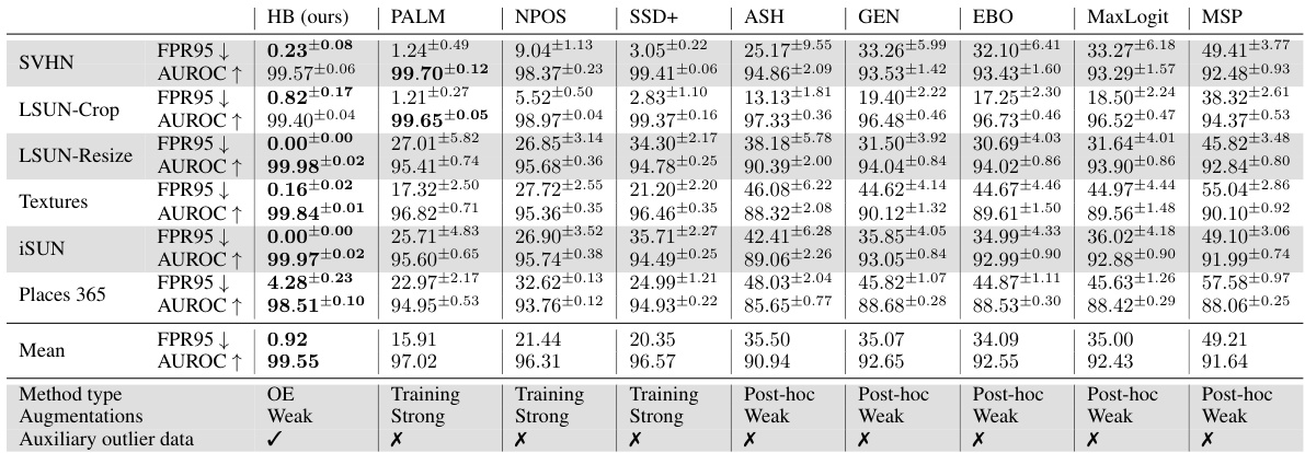
🔼 This table presents a comparison of the out-of-distribution (OOD) detection performance of Hopfield Boosting against several state-of-the-art methods on the CIFAR-10 dataset. The metrics used for comparison are the False Positive Rate at 95% True Positives (FPR95) and the Area Under the Receiver Operating Characteristic curve (AUROC). Lower FPR95 and higher AUROC values indicate better performance. Results are shown for several OOD datasets and are averaged over five independent training runs to provide an estimate of the standard deviation.
read the caption
Table 1: OOD detection performance on CIFAR-10. We compare results from Hopfield Boosting, DOS (Jiang et al., 2024), DOE (Wang et al., 2023b), DivOE (Zhu et al., 2023), DAL (Wang et al., 2023a), MixOE (Zhang et al., 2023b), POEM (Ming et al., 2022), EBO-OE (Liu et al., 2020), and MSP-OE (Hendrycks et al., 2019b) on ResNet-18. ↓ indicates “lower is better” and ↑ “higher is better”. All values in %. Standard deviations are estimated across five training runs.
Full paper#
