↗ OpenReview ↗ NeurIPS Homepage ↗ Chat
TL;DR#
Traditional numerical methods for solving Partial Differential Equations (PDEs) are computationally expensive and require significant expertise. Neural operators offer a data-driven alternative, learning the relationship between inputs and outputs without explicit equations. However, existing neural operators often suffer from high computational costs, particularly when dealing with large datasets. This limitation hinders their applicability to complex, real-world scenarios.
This paper introduces the Latent Neural Operator (LNO) to overcome these challenges. LNO leverages a latent space to reduce computational complexity while maintaining accuracy. It introduces a novel Physics-Cross-Attention (PhCA) module for efficient data transformation between the original space and the latent space, allowing for accurate predictions and interpolation/extrapolation. The experimental results demonstrate that LNO significantly improves computational efficiency (faster training and reduced memory usage) and achieves state-of-the-art accuracy on several benchmark problems. The method also shows promise for solving inverse PDE problems.
Key Takeaways#
Why does it matter?#
This paper is crucial for researchers working with partial differential equations (PDEs). It significantly improves the efficiency and accuracy of solving both forward and inverse PDE problems, offering a new paradigm for various scientific and engineering applications. The introduction of the Latent Neural Operator (LNO) opens exciting new avenues for research in this domain, particularly concerning the computational efficiency and generalization of neural operator methods. Furthermore, the LNO’s ability to handle inverse problems is a major step forward, addressing a significant challenge in the field.
Visual Insights#

The figure illustrates the architecture of the Latent Neural Operator (LNO), a model designed for solving both forward and inverse Partial Differential Equation (PDE) problems. The LNO consists of four main modules: an embedding layer, an encoder, a series of Transformer blocks for operator learning in latent space, and a decoder. The embedding layer transforms the input function data into higher-dimensional representations that consider both spatial coordinates and physical quantity values. The encoder utilizes Physics-Cross-Attention (PhCA) to map the input from geometric space to a learnable latent space. Transformer blocks then operate on this latent representation to learn the underlying PDE operator. The decoder uses PhCA to transform the latent representation back to geometric space, allowing prediction at any arbitrary point. This architecture is designed for improved accuracy and efficiency, particularly for inverse problems where interpolation and extrapolation are crucial.
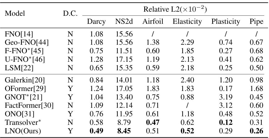
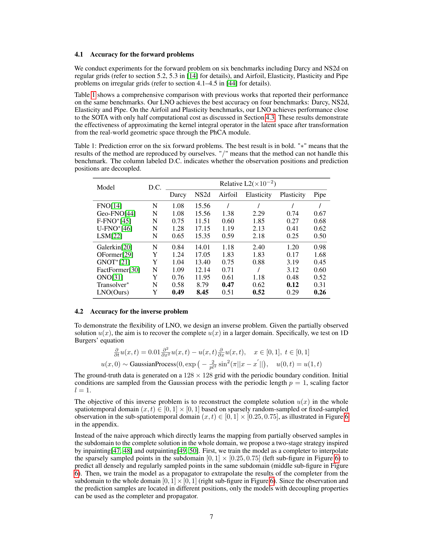
This table compares the prediction accuracy of different neural operator models on six benchmark problems for solving forward partial differential equations (PDEs). The accuracy is measured by the relative L2 error. The table shows the performance of various models, including the proposed Latent Neural Operator (LNO), highlighting LNO’s superior performance on most benchmarks and its efficiency in reducing computational cost. The ‘D.C.’ column indicates whether a model decouples observation and prediction positions, a key feature of the proposed LNO.
In-depth insights#
Latent PDE Solver#
A latent PDE solver is a powerful technique that leverages the power of neural networks to solve partial differential equations (PDEs) more efficiently than traditional methods. The core idea is to transform the PDE problem from its original high-dimensional geometric space into a lower-dimensional latent space. This dimensionality reduction significantly decreases computational cost and memory usage, particularly beneficial for large-scale PDEs. Within the latent space, a neural network, typically employing transformer architectures, learns the solution operator mapping inputs to outputs. After solving in the latent space, the solution is decoded back to the original geometric space, allowing for flexible prediction at arbitrary locations, not just at those defined in training. This flexibility is crucial for applications like interpolation and extrapolation, and particularly valuable for solving inverse PDE problems. A major advantage is the capacity to handle irregular geometries and complex boundary conditions, which would be challenging for traditional numerical methods. However, careful consideration must be given to the design of the latent space representation and the choice of neural network architecture to ensure the accuracy and stability of the solutions obtained. Furthermore, generalizability to unseen conditions and the interpretability of the learned operator remain active areas of research. The development of efficient encoding and decoding mechanisms is also key to the success of latent PDE solvers.
Physics-Cross-Attention#
The proposed Physics-Cross-Attention (PhCA) module is a crucial innovation in the Latent Neural Operator (LNO) framework, designed to efficiently and effectively map data between the geometric space and a learnable latent space. PhCA’s key strength lies in its decoupling of input and output sample locations, allowing for flexible prediction at arbitrary positions, unlike methods restricted to training locations. This is particularly beneficial for inverse problems needing extrapolation and interpolation. By employing a cross-attention mechanism, PhCA learns the optimal transformation between spaces, avoiding predefined latent spaces (like frequency domains) and enhancing the model’s adaptability to diverse PDE problems. The learnable latent space significantly reduces computational costs, as the model processes a smaller representation of the data, improving both training speed and memory efficiency. Moreover, sharing parameters between the encoder and decoder PhCA modules ensures consistency and reduces the number of parameters, further streamlining the overall LNO framework. The integration of PhCA as the core transformational component within LNO showcases a clear advancement in operator learning for PDEs.
Efficiency Gains#
The research paper highlights significant efficiency gains achieved by the proposed Latent Neural Operator (LNO) model. LNO reduces GPU memory consumption by 50%, a substantial improvement compared to existing methods. This reduction is attributed to the model’s design, which processes data in the latent space, decreasing the computational burden associated with large datasets. Furthermore, training time is accelerated by a factor of 1.8x, demonstrating a remarkable increase in training efficiency. This speedup is directly linked to the reduced memory footprint and computational complexity resulting from the latent space operation. These efficiency enhancements are crucial for scaling up the application of neural operators to complex, high-dimensional PDE problems. The paper presents these gains as key advantages of LNO, making it a more practical and scalable solution for real-world applications. The improvement in efficiency complements the model’s high accuracy, positioning LNO as a strong contender for various scientific and engineering applications requiring efficient PDE solutions.
Inverse Problem#
The section on inverse problems highlights the significance of this class of PDEs in diverse fields like medical imaging and geological sensing. It emphasizes the challenges posed by inverse problems, noting that traditional numerical methods often struggle with these due to the ill-posed nature of many inverse problems. The discussion underscores the need for robust and efficient methods capable of handling incomplete or noisy data, typical of real-world scenarios. The text then transitions to the application of neural networks to solve inverse problems, pointing out the flexibility and efficiency that these models can offer, especially when compared to classical techniques. Specifically, the paper advocates for the use of neural operator models, given their capabilities of learning implicit relationships in data and their ability to handle complex geometries. This section, therefore, lays a foundation for the core contribution of the paper—addressing the challenges of inverse problems with a novel neural operator technique.
Future Scope#
The paper’s focus on efficiently solving both forward and inverse PDE problems using the Latent Neural Operator (LNO) opens several promising avenues for future research. Extending LNO’s capabilities to handle more complex PDE types such as those with higher-order derivatives, stochastic terms, or highly nonlinear behavior would be a significant advancement. Further investigation is needed into the optimal design and learning of the latent space within LNO, potentially exploring alternative methods beyond the Physics-Cross-Attention mechanism. Improving the model’s generalizability and robustness across varied datasets and problem setups is another crucial area. This might involve incorporating techniques for handling uncertainties, non-uniform spatial resolutions, and adaptive learning rates. Finally, developing a comprehensive theoretical understanding of LNO’s properties, convergence, and approximation capabilities would be essential for enhancing its reliability and predictive accuracy. Exploring the integration of LNO with other advanced machine learning techniques, like generative models or Bayesian methods, could unlock new functionalities and enhance the framework’s ability to deal with incomplete or noisy data. This could lead to more robust and insightful solutions to a wide range of complex scientific and engineering problems.
More visual insights#
More on figures

This figure illustrates the Physics-Cross-Attention (PhCA) module, a core component of the Latent Neural Operator (LNO). The PhCA module acts as both an encoder and decoder, transforming data representations between the real-world geometric space and a learnable latent space. The diagram shows the process for both the encoder (left) and decoder (right). In the encoder, input position embeddings (X) and value embeddings (Y) are processed by the attention projector, along with learnable query positions. The resulting latent representation (Z0) is then passed to subsequent processing stages. The decoder performs the inverse transformation, mapping the latent space representation (ZL) back to the real-world geometric space.
This figure illustrates the detailed architecture of the Physics-Cross-Attention (PhCA) module, which is a core component of the Latent Neural Operator (LNO). The PhCA module acts as both an encoder and decoder, transforming data representations between the real-world geometric space and a learnable latent space. The figure displays the process of encoding the input function into the latent space and the subsequent decoding of the output function back to the real-world space, highlighting the decoupling property and the learnable latent space. Specifically, it shows how the input’s position and quantity values are encoded into the latent space by the encoder’s PhCA, and then how the decoder’s PhCA utilizes learnable latent space positions to produce the corresponding output function. The learnable matrices (W1, W2) in the encoder and decoder share the same parameters for efficiency, which is different from the Transolver architecture.
This figure illustrates the overall architecture of the Latent Neural Operator (LNO) model. It consists of four main modules: an embedding layer that converts the input data into a higher-dimensional representation; an encoder that transforms the input data into a learnable latent space using the Physics-Cross-Attention (PhCA) mechanism; a series of Transformer blocks that learn the PDE operator within the latent space; and a decoder that transforms the output from the latent space back into the original geometric space, also using the PhCA mechanism. The figure clearly shows the flow of data through these modules, including the input function, observation positions, prediction positions, and output function. The PhCA module is highlighted as a key component of the LNO, responsible for the transformation between the geometric space and latent space, and enabling the model to operate on latent representations of input/output functions.
This figure shows the overall architecture of the Latent Neural Operator (LNO). The LNO consists of four main modules: an embedding layer, an encoder using Physics-Cross-Attention (PhCA) to transform data to a latent space, a series of Transformer blocks to learn the operator in the latent space, and a decoder (also using PhCA) to transform data back to the real-world geometric space. The figure highlights the flow of data through these modules, starting with the input function and ending with the output function. The key innovation is the use of the PhCA module which decouples input and output sample locations, enabling flexibility in predicting values at positions not seen during training.

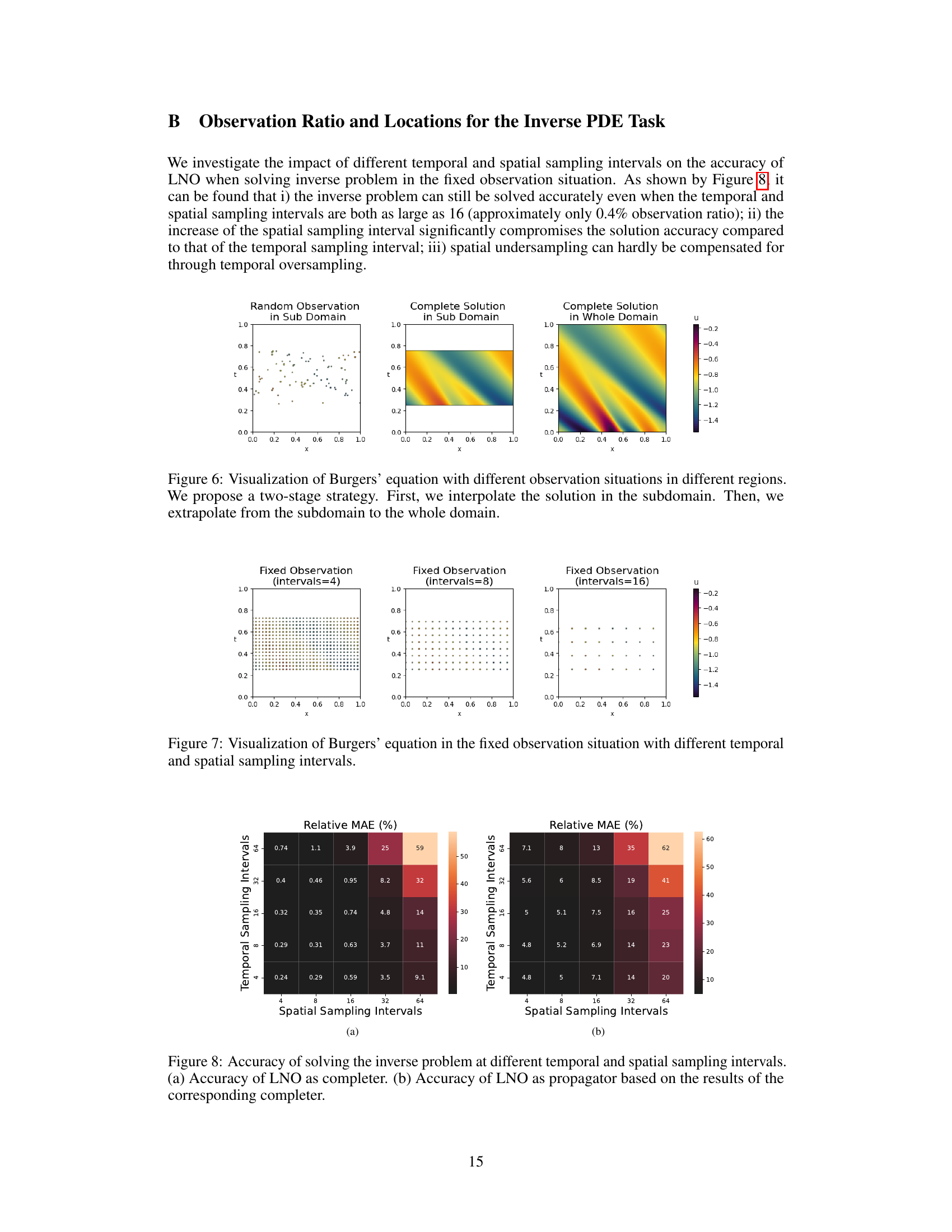
This figure visualizes the results of solving the Burgers’ equation using different observation strategies. The leftmost panel shows a random observation in a subdomain, the middle panel shows the complete solution interpolated within the same subdomain, and the rightmost panel shows the complete solution extrapolated to the entire domain. The figure illustrates the two-stage approach (interpolation followed by extrapolation) used in the inverse problem to reconstruct the solution from sparse observations.

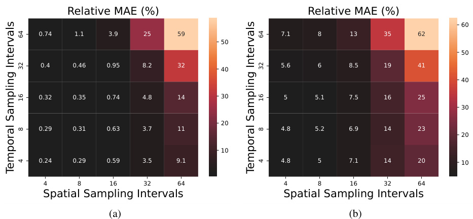
This figure visualizes the results of solving the Burgers’ equation using different temporal and spatial sampling intervals in a fixed observation scenario. It demonstrates how the accuracy of the solution is affected by varying the density of the observed data points. The figure shows three subplots, each representing a different level of sampling density (intervals=4, 8, and 16), and a colorbar indicating the values of the solution, u. Each subplot displays the spatial and temporal locations of the observed data points as small dots. The plot shows that increasing sampling interval decreases the accuracy of the result in the extrapolation region, especially the temporal sampling interval.
This figure illustrates the Physics-Cross-Attention (PhCA) mechanism used in both the encoder and decoder of the Latent Neural Operator (LNO). The encoder transforms data from the geometric space to the latent space, while the decoder performs the reverse transformation. The diagram highlights the key components: the attention mechanism (softmax), projection layers, and the interaction between query (H or P), key (X), and value (Y) matrices. The use of learnable parameters in these matrices emphasizes the data-driven learning aspect of PhCA, allowing the model to automatically learn efficient mappings between function spaces.
More on tables

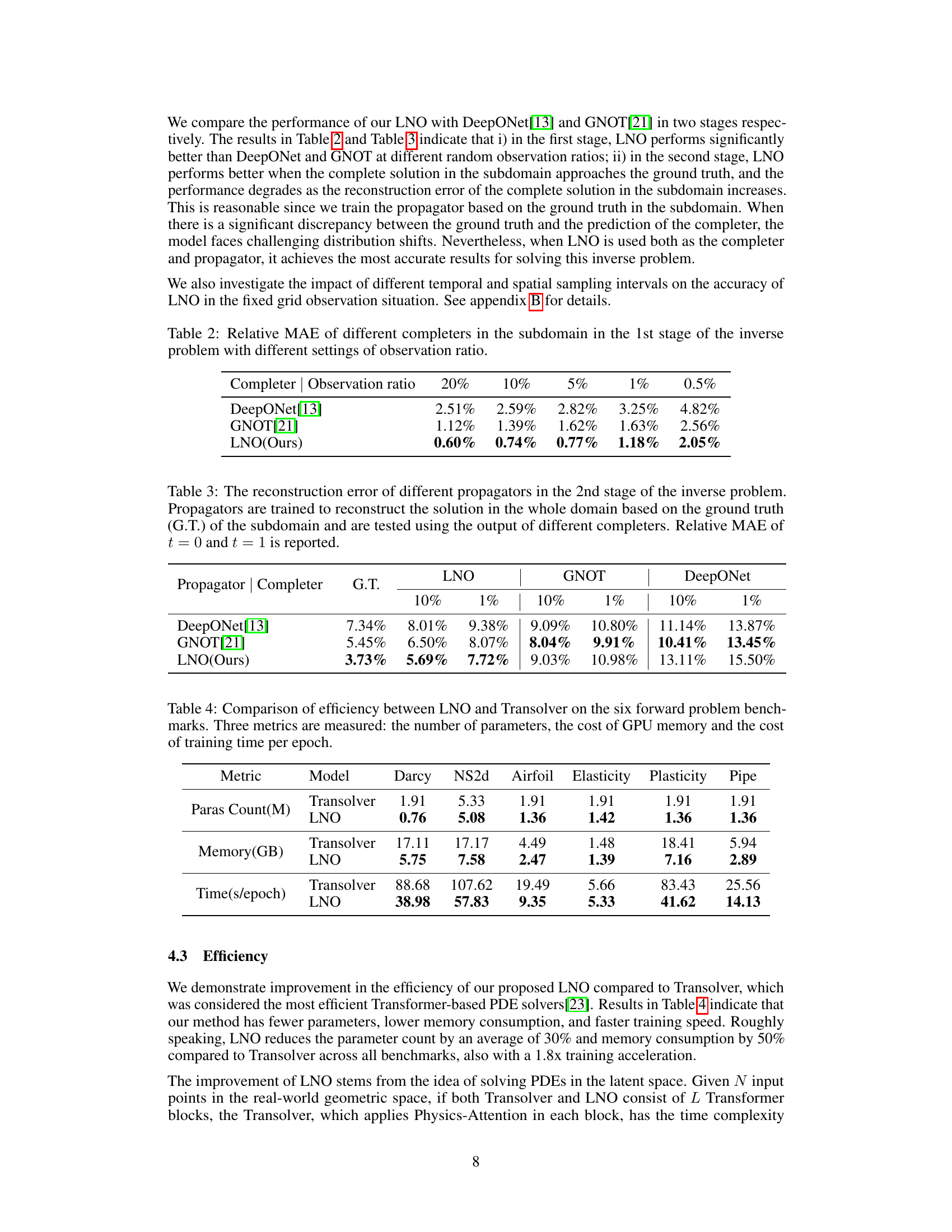
This table presents the relative Mean Absolute Error (MAE) achieved by three different models (DeepONet, GNOT, and the proposed LNO) in the first stage of an inverse problem. The first stage involves reconstructing a complete solution within a subdomain using only a portion of the data. The table compares the performance of these models at varying observation ratios (20%, 10%, 5%, 1%, and 0.5%). Lower MAE values indicate better performance.

This table compares the reconstruction error of three different propagators (DeepONet, GNOT, and LNO) in the second stage of an inverse problem. The propagators aim to reconstruct the complete solution across the entire domain using the ground truth from a subdomain. The error is evaluated using the Relative Mean Absolute Error (MAE) at times t=0 and t=1, and is shown for different observation ratios (10%, 1%, 0.5%) in the initial subdomain used by the completer.

This table presents a comparison of the prediction error achieved by various models on six benchmark problems for solving forward partial differential equations. The models are evaluated using the Relative L2 error metric. The table indicates which models allow decoupling of observation and prediction positions and highlights the best-performing model for each benchmark. The table includes results reproduced by the authors as well as results from other publications.

This table compares the prediction error (Relative L2 error) of the proposed Latent Neural Operator (LNO) model against several other state-of-the-art models on six benchmark forward problems (Darcy, NS2d, Airfoil, Elasticity, Plasticity, and Pipe). The table shows the relative L2 error for each method and benchmark, indicating the accuracy of each model in solving the specific problem. The ‘D.C.’ column indicates whether each method decouples the observation and prediction positions. The best performance for each benchmark is highlighted in bold.

This table presents a comparison of the prediction error achieved by various models on six forward problems. The models are evaluated based on their relative L2 error. The table includes whether the method’s results were reproduced by the authors or if it was unable to handle a specific benchmark. A key aspect highlighted is whether the models decouple observation and prediction positions, indicating the flexibility and generalizability of the approach.

This table compares the prediction accuracy of the proposed Latent Neural Operator (LNO) against other state-of-the-art methods across six benchmark datasets for solving forward Partial Differential Equations (PDEs). The results are presented as relative L2 errors, indicating the difference between the predicted and ground truth solutions. The table also notes whether each method decouples observation and prediction positions (D.C.) and indicates which results were reproduced by the authors of the paper.

This table compares the prediction accuracy (Relative L2 error) of various models on six benchmark PDE problems. The model LNO (Latent Neural Operator) is compared against several other state-of-the-art neural operator models, showing its accuracy and competitive performance compared to other existing methods. The table also highlights whether each method decouples observation and prediction positions, a key feature of LNO, and indicates where results were reproduced by the authors or are unavailable from the original sources.

This table shows the reconstruction error of different propagators in the second stage of the inverse problem. The propagators are trained using the ground truth of the subdomain and tested using different completers’ outputs. The relative mean absolute error (MAE) at t=0 and t=1 are shown for each combination of propagator and completer, providing insights into the accuracy of reconstructing the complete solution.

This table presents a comparison of the prediction error achieved by various models on six benchmark problems for solving forward partial differential equations (PDEs). The models’ accuracy is measured using the relative L2 error. The table also indicates whether each model decouples the observation positions from prediction positions. This decoupling is a key feature of the proposed Latent Neural Operator (LNO) and allows it to perform interpolation and extrapolation.
Full paper#
