Randomized algorithms and PAC bounds for inverse reinforcement learning in continuous spaces

↗ OpenReview ↗ NeurIPS Homepage ↗ Chat

TL;DR

#

Key Takeaways

#

Why does it matter?

#

This paper is crucial for researchers in reinforcement learning and related fields because it offers novel theoretical guarantees and practical algorithms for inverse reinforcement learning in continuous spaces. This addresses a major limitation of existing methods and opens avenues for more robust and reliable applications of IRL in various real-world scenarios such as robotics and autonomous systems.

Visual Insights

#

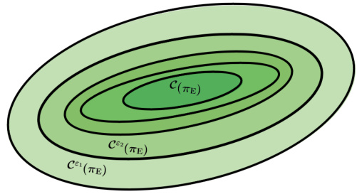
The figure illustrates Theorem 3.1, which characterizes the inverse feasibility set. It shows a series of nested ellipses, where each ellipse represents the ε-inverse feasibility set Cε(πε) for a different value of ε. The innermost, dark green ellipse represents the inverse feasibility set C(πε), which contains cost functions for which the expert policy πε is optimal. As ε increases, the ellipses grow larger, representing a larger set of nearly optimal cost functions Cε(πε). The figure shows that as epsilon gets larger, more cost functions are considered ’nearly’ optimal.

In-depth insights

#

Continuous IRL

#

Continuous Inverse Reinforcement Learning (IRL) tackles the challenge of learning reward functions in continuous state and action spaces. This is a significant departure from traditional IRL, which often simplifies the problem by discretizing the environment. The complexity arises from the infinite dimensionality of the problem. Methods addressing this often employ function approximation techniques, such as linear or nonlinear models, to represent the reward function. This introduces approximation errors, and rigorous analysis is needed to bound these errors and guarantee solution quality. Sampling-based approaches are commonly used to handle the infinite number of constraints in continuous MDPs, but require careful consideration of sample complexity to ensure reliable solutions. A key challenge is dealing with the inherent ill-posedness of IRL, where many reward functions can explain the same observed behavior, requiring regularization or constraints to find a meaningful solution. The core of continuous IRL research lies in developing efficient and theoretically sound algorithms that can effectively balance approximation errors with sample complexity.

PAC Bounds

#

PAC (Probably Approximately Correct) bounds are a cornerstone of computational learning theory, offering a rigorous framework for analyzing the sample complexity of learning algorithms. In the context of inverse reinforcement learning (IRL), PAC bounds provide valuable insights into the number of expert demonstrations needed to guarantee that a learned cost function approximates the true cost function within a specified error tolerance. A key strength of PAC analysis is its ability to quantify the trade-off between the desired accuracy of the learned model and the amount of data required. This is particularly useful in IRL where obtaining expert demonstrations can be costly or time-consuming. Effective PAC bounds for IRL are critical for evaluating the feasibility and efficiency of different IRL algorithms, allowing researchers to compare the sample complexity of various methods and make informed choices regarding data acquisition strategies. The development of tight PAC bounds for IRL in continuous state and action spaces remains a significant challenge. This is primarily because continuous spaces often result in infinite-dimensional optimization problems requiring sophisticated approximation techniques and sample complexity analysis.

Scenario Approach

#

The scenario approach, within the context of this research paper focusing on inverse reinforcement learning (IRL) in continuous spaces, is a randomized method used to address the computational intractability of infinite-dimensional linear programs arising from the problem formulation. It tackles the challenge by approximating the infinite constraints using a finite, randomly sampled subset of them. This approximation introduces a probabilistic element; the solution obtained is not guaranteed to be optimal but comes with probabilistic feasibility guarantees. These guarantees bound the probability that the approximate solution satisfies the true (infinite) constraints. The effectiveness of this approach hinges on the sample size (N) of the randomly selected constraints, demonstrating a trade-off between computational cost and accuracy. A larger N leads to higher confidence in the feasibility of the solution but increases computational demands. The theoretical analysis provides bounds on the required N for a desired level of confidence, highlighting the sample complexity of the scenario approach and its dependence on factors like desired accuracy and confidence levels. The paper significantly contributes by applying and analyzing the scenario approach in a continuous IRL context, filling a gap in existing IRL algorithms and providing theoretical justifications for its application. Moreover, it provides practical guidance on the choice of N, making this method potentially valuable for solving challenging IRL problems in real-world applications.

Sample Complexity

#

The concept of ‘sample complexity’ in the context of inverse reinforcement learning (IRL) is crucial because it quantifies the amount of data needed to learn an accurate reward function. The paper investigates sample complexity in continuous state and action spaces, a particularly challenging setting. This is important because many real-world problems naturally have continuous state and action spaces (e.g., robotics, autonomous driving). The authors explore the impact of various factors on sample complexity, such as the dimensionality of the state and action spaces, the richness of the function approximator used to model the reward, and the desired level of accuracy in the learned reward. Bounds on the error made when working with a finite sample of expert demonstrations are derived. This analysis helps to understand the trade-off between data collection effort and accuracy. The scenario approach is used for the theoretical analysis and provides probabilistic performance guarantees for approximation accuracy. The findings highlight the challenges posed by continuous state spaces, showing an exponential growth in sample complexity. This underscores the need for efficient data-gathering strategies and sophisticated approximation techniques to make IRL in continuous spaces practically feasible.

Future Work

#

Future research directions stemming from this work are multifaceted. Extending the theoretical framework to handle non-stationary expert policies and non-Lipschitz continuous dynamics is crucial for broader applicability. Investigating alternative regularization techniques beyond the L1 norm, and exploring ways to leverage prior knowledge about cost function structure (e.g., sparsity, smoothness) could significantly enhance the efficiency and robustness of the proposed methods. Developing more efficient algorithms for solving the semi-infinite programming problem, perhaps by exploiting problem structure or employing advanced optimization techniques, is vital. Addressing the curse of dimensionality, a major challenge in continuous spaces, could involve developing novel sampling strategies that intelligently focus on regions of high information content or utilizing advanced dimensionality reduction techniques. Finally, thorough empirical evaluation on a wider range of continuous control tasks is needed to validate the proposed approach and demonstrate its practical benefits.

More visual insights

#

More on figures

This figure illustrates the main steps of the proposed methodology. It starts with the inverse MDP problem, which is addressed using occupancy measures and linear duality to formulate an infinite-dimensional feasibility LP. This is then tackled by adding a normalization constraint and projecting onto features to create a regularized semi-infinite program. Constraint sampling is used to reduce this to a scenario convex program, which provides a scenario bound. Alternatively, a data-driven counterpart is used when only expert trajectories and a generative model are available. This also involves finite-sample analysis.

This figure presents the results of experiments using the Sampled Inverse Program (SIPN) to learn a cost function from data. Four subplots show the empirical confidence of the learnt cost function being within a given error bound (a), the objective function value of the SIPN program (b), the theoretical sample complexity according to Theorem 4.1 (c), and a comparison of the discounted cost under the learnt and expert policies (d).

This figure shows the results of applying the Sampled Inverse Program (SIPN) for different sample sizes (N). It contains four subplots. Subplot (a) shows the empirical probability of the estimated cost function being in the feasibility set for different values of N and ε. Subplot (b) displays the average objective value of the SIPN with standard deviation for different values of N. Subplot (c) shows the theoretical sample complexity bounds. Subplot (d) compares the discounted long-run costs for the average learnt cost and optimal policy.

Figure 4 presents the results of the Sampled Inverse Program SIPN,m,n,k, an algorithm designed to estimate the cost function with unknown transition kernels. Plot (a) displays the empirical probability that the learned cost function belongs to a specific feasibility set, demonstrating how increasing sample size N and reducing the error tolerance ε improves the accuracy of cost estimation. Plot (b) shows the theoretical lower bound of k (number of calls to the generative model per constraint), which increases with N and ε, indicating a trade-off between sample size and computational cost.

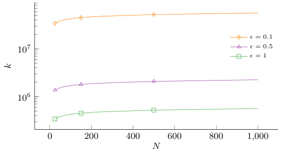
Figure 3 shows the results of the Sampled Inverse Program (SIPN) experiments. It presents four plots illustrating different aspects of the algorithm’s performance. Plot (a) shows the empirical probability of the learned cost function being within the feasibility set for different sample sizes and error tolerances. Plot (b) displays the average objective function value of the SIPN across multiple runs, with error bars representing the standard deviation. Plot (c) visualizes the theoretical sample complexity, comparing it to the empirical results. Plot (d) compares the long-run cost under the expert policy and the learned cost function.

Full paper

#