↗ OpenReview ↗ NeurIPS Homepage ↗ Hugging Face ↗ Chat
TL;DR#
Training large language models is computationally expensive, often constrained by memory limitations. Pipeline parallelism, a model-parallelism strategy, splits the model across devices, improving memory efficiency, but it suffers from pipeline bubbles (idle time) and high activation memory. Existing methods lack systematic approaches to schedule pipeline operations efficiently.
This paper presents a new framework that systematizes pipeline scheduling using reusable building blocks. The authors demonstrate that the lifespan of these blocks directly determines peak activation memory. Leveraging this insight, they introduce a family of memory-efficient building blocks. These blocks reduce peak activation memory by half or even a third compared to the state-of-the-art 1F1B approach, without sacrificing training speed and even achieving near-zero bubbles. Experiments show significant improvements (7-55%) in throughput compared to 1F1B in different settings.
Key Takeaways#
Why does it matter?#
This paper is crucial for researchers working on large language model training because it introduces a novel framework for designing pipeline schedules that significantly improves memory efficiency without sacrificing throughput. This directly addresses a major bottleneck in training massive models and opens avenues for optimizing distributed training strategies. The open-sourced implementation further enhances its impact on the research community.
Visual Insights#

This figure illustrates the concept of building a pipeline by repeating a basic building block. It shows how pipelines, such as 1F1B and Eager 1F1B, can be constructed by repeating these blocks. The figure also demonstrates how squeezing redundant bubbles from the repeated blocks can lead to a more efficient pipeline. The different shades of gray represent different microbatches in the pipeline.

This table summarizes the peak memory and number of bubbles for different pipeline building blocks (1F1B, V-Min, V-Half, and V-ZB). It shows how the proposed V-shaped building blocks achieve significant memory reduction compared to the baseline 1F1B, while also controlling the number of bubbles. The parameters δ⁰ and δ¹ represent offsets within the building blocks.
In-depth insights#
Pipeline Decomp#
The concept of “Pipeline Decomp,” or pipeline decomposition, in the context of parallel computing, involves breaking down a large computational task into smaller, manageable subtasks that can be executed concurrently across multiple processing units. This is crucial for optimizing the efficiency of pipeline parallelism, especially when dealing with large language models (LLMs) where memory constraints are a significant bottleneck. Effective pipeline decomposition strategies aim to balance memory usage across pipeline stages while minimizing inter-stage communication and idle time (pipeline bubbles). Careful consideration of the lifespan of individual pipeline stages is essential for optimizing memory efficiency as it directly impacts peak memory consumption. Advanced decomposition techniques might leverage techniques like activation recomputation or memory-efficient building blocks to further improve memory efficiency and throughput.
Memory Control#
The concept of ‘Memory Control’ in large language model training, particularly within the context of pipeline parallelism, is crucial for efficiency. Minimizing peak activation memory is a primary goal, as it directly impacts the scalability of training. The paper explores this by framing pipeline schedules as repeating building blocks, where the lifespan of the block determines peak memory. This insight reveals that existing methods are often inefficient. Controllable memory building blocks are introduced, offering the ability to reduce peak memory to 1/2 or even 1/3 of the baseline (1F1B) without significant throughput loss. Strategies like V-Shape building blocks balance memory usage across devices. A key finding is the direct link between the lifespan of these blocks and the activation memory, enabling a more systematic approach to pipeline schedule design. The introduction of an adaptive scheduler further refines memory control by searching for optimal offset combinations, achieving near-zero pipeline bubbles while respecting memory constraints. This work demonstrates that carefully designed pipeline parallelism significantly improves training efficiency by controlling and optimizing memory usage.
V-Shape Blocks#
The proposed V-Shape Blocks represent a novel approach to pipeline parallelism, directly addressing the memory inefficiency prevalent in existing methods. The core idea is to balance memory usage across pipeline stages by strategically placing stages with long and short lifespans together. This is achieved by carefully controlling the offsets between forward and backward passes within the building block. The V-Shape configuration, with its mirrored structure, facilitates this balanced memory distribution and leads to significant memory savings—up to a reduction of activation memory to 1/3 of 1F1B without sacrificing throughput. Further investigation of different offset combinations within the V-Shape framework offers potential for further optimization and control over both memory consumption and pipeline efficiency. This design enhances memory efficiency without introducing significant communication overhead, making it suitable for training large language models where memory is a critical constraint.
Bubble Analysis#
The section on ‘Bubble Analysis’ would delve into the phenomenon of pipeline bubbles in parallel processing, specifically within the context of large language model training. It would likely start by defining pipeline bubbles as periods of inactivity or underutilization of computational resources in a pipeline due to timing mismatches between stages. The analysis would then explore how bubble formation relates to the design of the pipeline’s building blocks and their impact on overall training efficiency. Key factors such as the duration of forward and backward passes, the sizes of microbatches, and the synchronization mechanisms employed would be thoroughly examined. The analysis could also include mathematical models or simulations to quantify the frequency and duration of bubbles under different operating conditions. Furthermore, the analysis could explore strategies for minimizing bubbles, perhaps through careful scheduling, memory optimization techniques, or asynchronous operation. Finally, the discussion might incorporate results from experimental evaluations demonstrating the effectiveness of proposed bubble mitigation methods, highlighting the trade-offs between throughput and memory utilization. A central theme would be how to balance the desire for high throughput with the need to keep memory consumption within acceptable limits.
Future Work#
The authors outline future research directions focusing on further enhancing memory efficiency in pipeline parallelism. They plan to explore more sophisticated scheduling techniques to mitigate the limitations of their current V-Min approach, which suffers from increased bubble rates as the number of microbatches grows. Addressing this issue is crucial for maintaining scalability. Additionally, they aim to investigate the use of continuous offsets in their scheduling framework, which could potentially lead to even finer-grained control over memory usage and allow for more flexibility in optimizing pipeline efficiency. The investigation of continuous offsets offers a promising path towards more advanced and robust memory management. This future work demonstrates a commitment to pushing the boundaries of pipeline parallelism, particularly in the context of very large language models where memory constraints are often a major bottleneck. The focus on both bubble rate reduction and memory optimization highlights a balanced and pragmatic approach to future research.
More visual insights#
More on figures

This figure compares two different building block designs for pipeline parallelism: Parallel and V-Shape. The Parallel design shows an imbalanced memory usage, with the first device having a memory bottleneck. The V-Shape design, in contrast, achieves a balanced peak memory across all devices, improving memory efficiency. The lifespans of each stage are represented by the colored blocks.
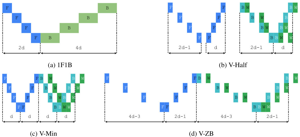
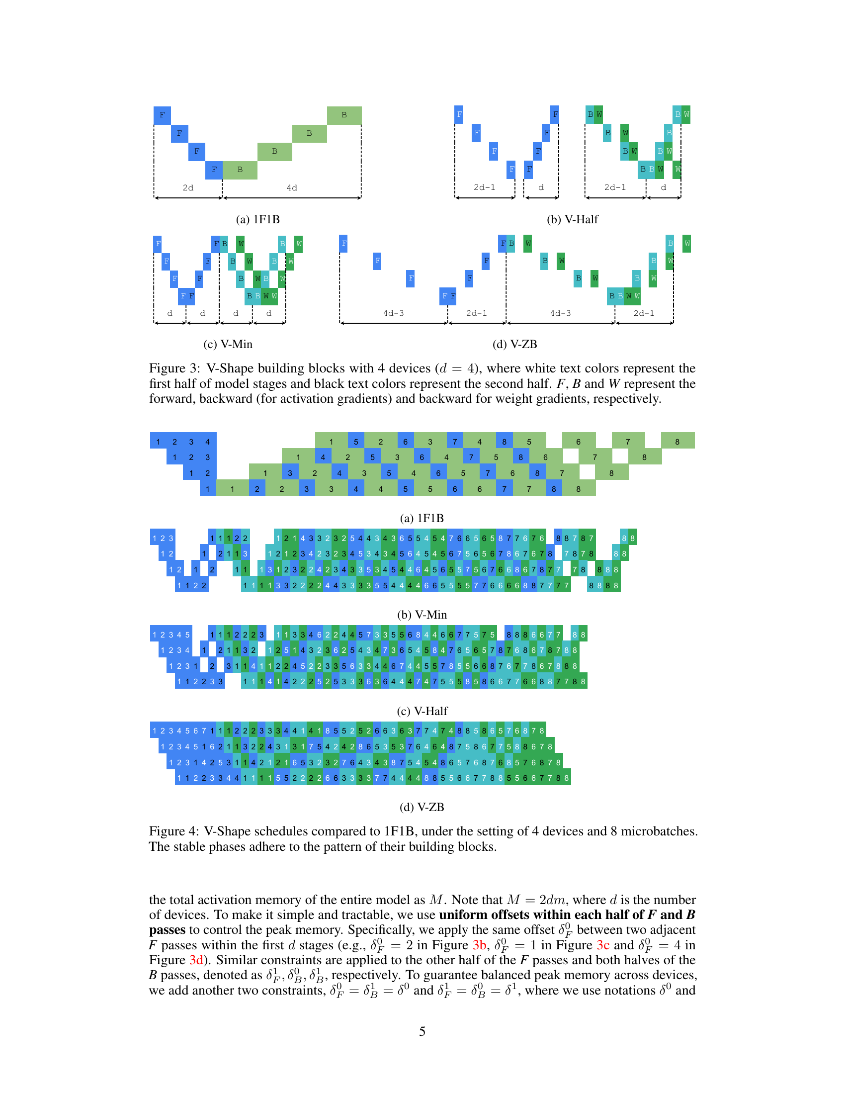
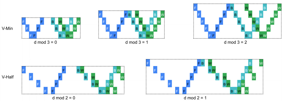
This figure shows the building blocks of three different V-shape pipeline schedules (V-Min, V-Half, and V-ZB) with 4 devices. Each block is made of forward (F), backward for activations (B), and backward for weights (W) passes. The arrangement of these passes determines the memory efficiency and the number of pipeline bubbles. White text represents the first half of the model stages, while black text represents the second half. The differences in the arrangement of passes across the three V-shape blocks illustrate how different memory consumption and bubble rates can be achieved by changing the scheduling of forward and backward passes.

This figure shows four different V-Shape building blocks designed for pipeline parallelism with four devices. Each building block is a sequence of forward (F), backward for activations (B), and backward for weights (W) passes. The blocks differ in the arrangement and offsets of these passes, which affects their memory efficiency and the resulting pipeline schedule. The ‘V-Shape’ refers to the arrangement of passes, where the first half of stages uses one pattern and the second half mirrors this pattern, aiming for balanced memory consumption across all devices.

This figure showcases different V-Shape building block variations with 4 devices. The white text represents the first half of the model’s stages, and black text represents the second half. F, B, and W denote forward, backward (for activation gradients), and backward (for weight gradients) passes, respectively. The variations illustrate how different arrangements of these passes impact memory efficiency and pipeline design.

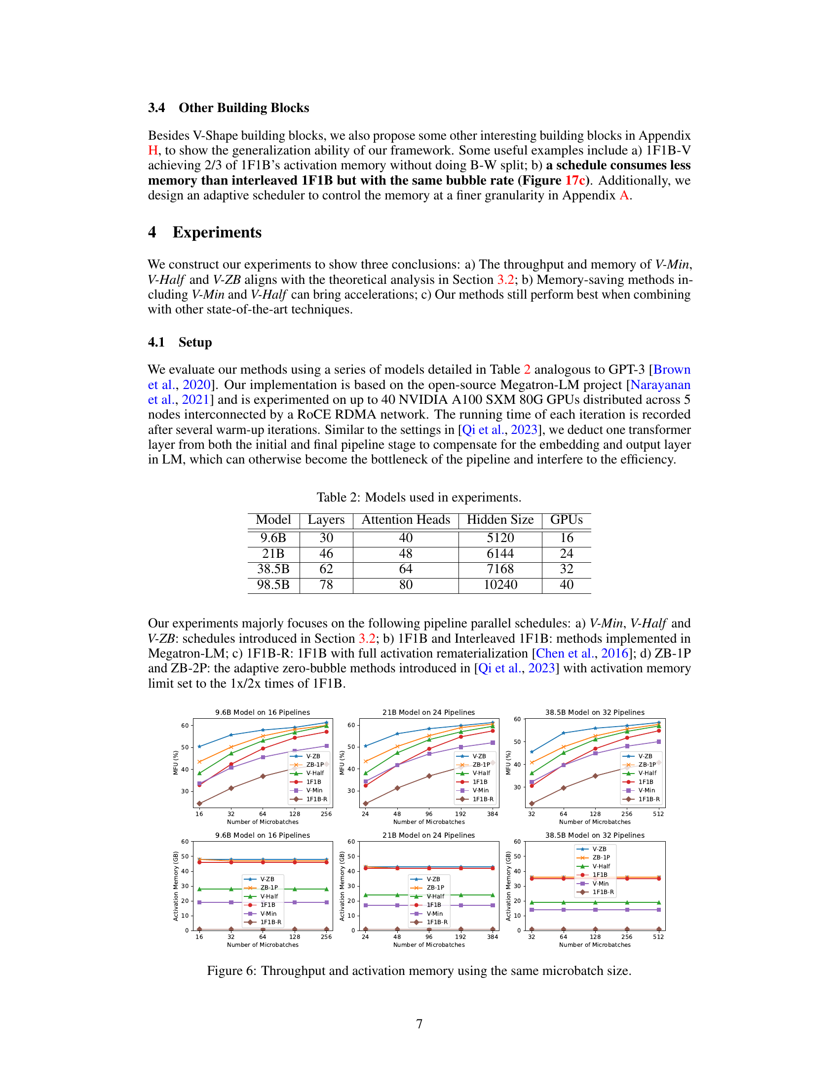
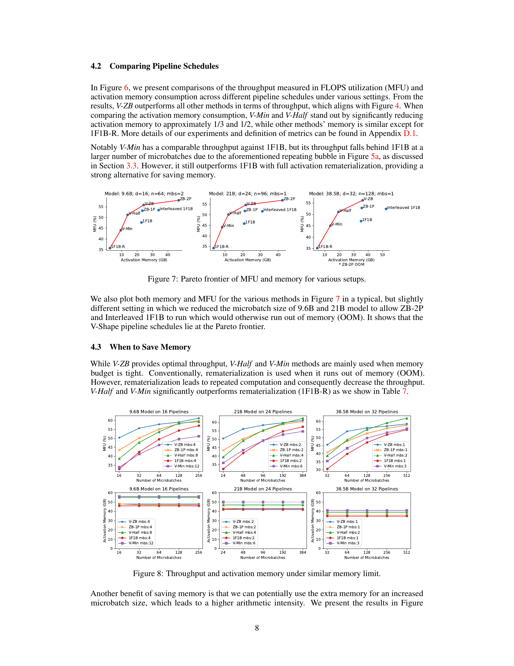
This figure compares different pipeline parallel schedules (V-ZB, ZB-1P, V-Half, 1F1B, V-Min, 1F1B-R) across three different model sizes (9.6B, 21B, 38.5B) and varying numbers of microbatches. The top row shows the throughput (MFU, or FLOPS utilization), while the bottom row shows the activation memory used. The results demonstrate the performance and memory efficiency trade-offs of each schedule.

This figure compares the throughput (measured in FLOPS utilization or MFU) and activation memory consumption across different pipeline parallel schedules. It shows the results for three different model sizes (9.6B, 21B, and 38.5B parameters) each with varying numbers of microbatches. The figure demonstrates that V-ZB consistently outperforms other methods in terms of throughput, while V-Min and V-Half significantly reduce activation memory compared to 1F1B.
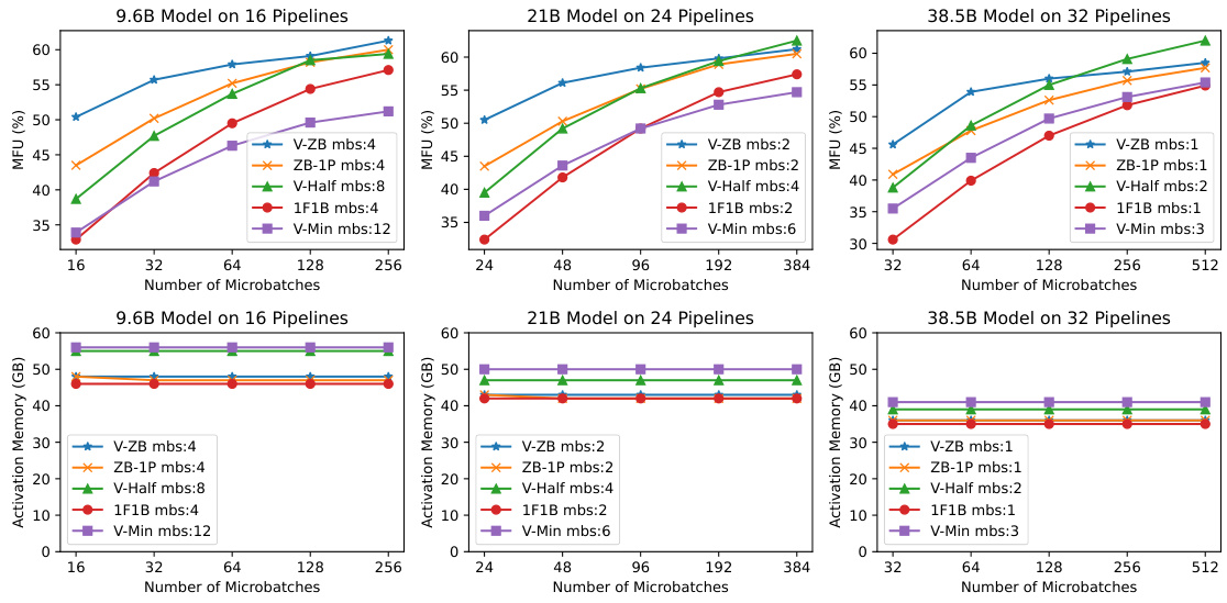
This figure compares the throughput (measured in FLOPS utilization or MFU) and activation memory consumption of different pipeline schedules (V-ZB, ZB-1P, V-Half, 1F1B, V-Min, and 1F1B-R) under various settings (9.6B, 21B, and 38.5B models) and with different numbers of microbatches. It visually demonstrates the trade-off between memory and throughput and illustrates the improvements achieved by the proposed methods.

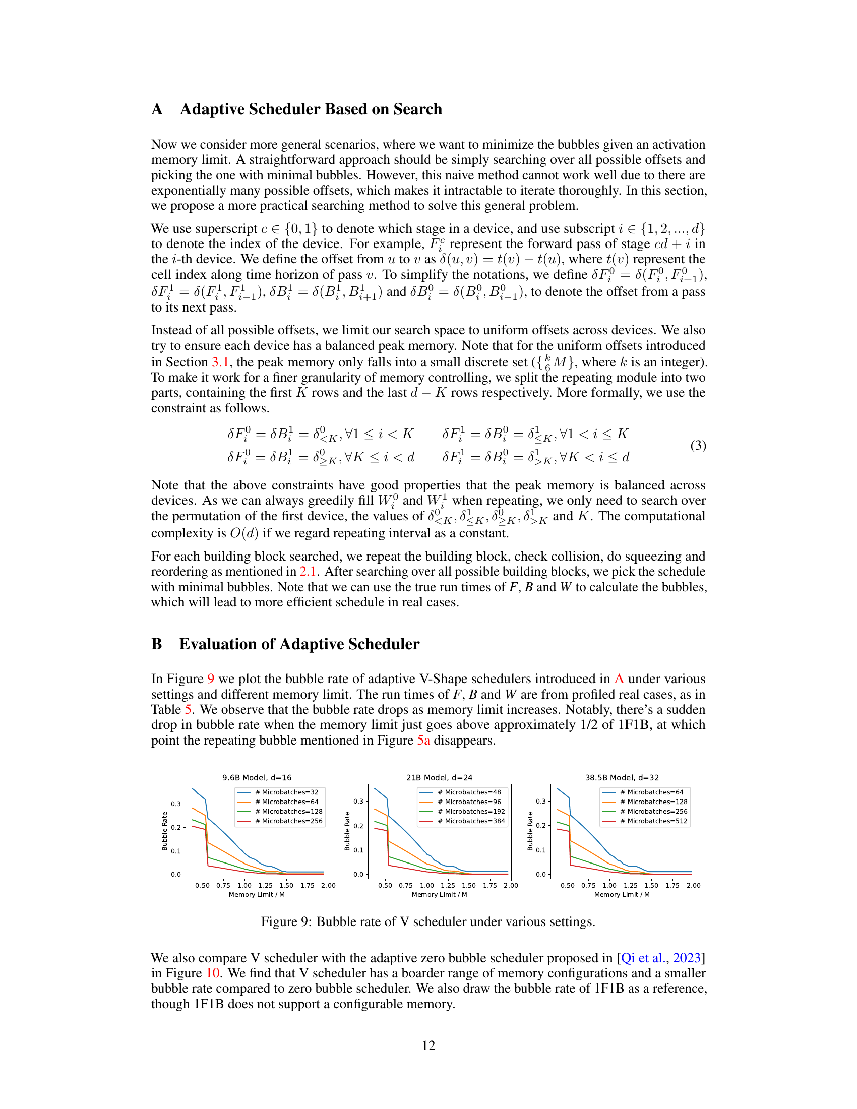
This figure shows the bubble rate of the adaptive V-Shape scheduler under various settings and different memory limits. The x-axis represents the memory limit as a fraction of the memory used by the 1F1B baseline. The y-axis represents the bubble rate. Different lines represent different numbers of microbatches. The figure shows that the bubble rate drops significantly as the memory limit increases. There is a sudden drop in the bubble rate when the memory limit is just above approximately 1/2 of 1F1B, indicating that the repeating bubbles observed in Figure 5a disappear.

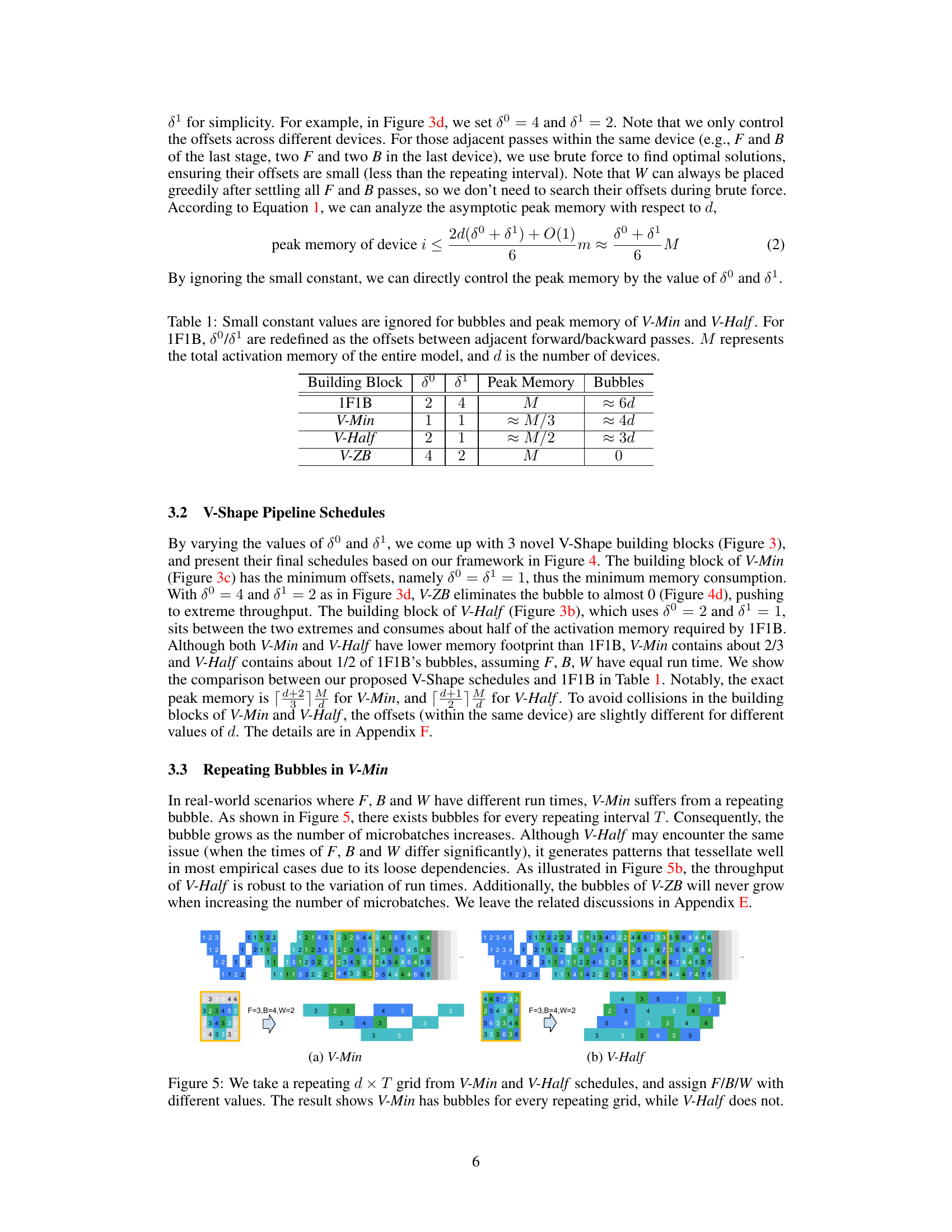
This figure compares different pipeline schedules, namely 1F1B, V-Min, V-Half, and V-ZB, using 4 devices and 8 microbatches. The visualization shows the sequence of forward (F), backward (B), and weight update (W) passes across the different stages and devices over the 8 microbatches. The stable phase (the middle section of each schedule) shows the repeating pattern, highlighting the difference between each method’s memory usage and scheduling efficiency.
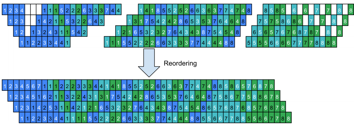
This figure compares different pipeline schedules: 1F1B, V-Min, V-Half, and V-ZB. Each schedule is visualized as a sequence of forward (F), backward for activations (B), and backward for weights (W) passes across 4 devices over 8 microbatches. The visualization highlights how each schedule arranges these passes to form building blocks that repeat over time. The goal is to reduce memory usage and pipeline bubbles while maintaining high throughput. The V-shaped schedules (V-Min, V-Half, V-ZB) show different memory optimization strategies compared to the 1F1B baseline.
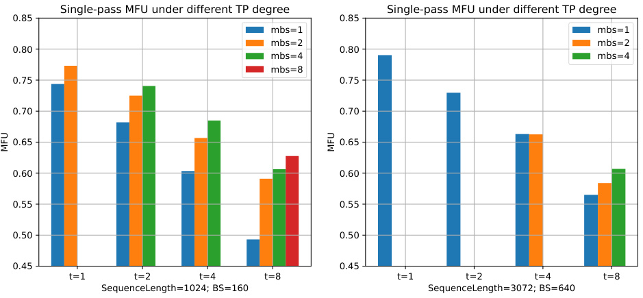
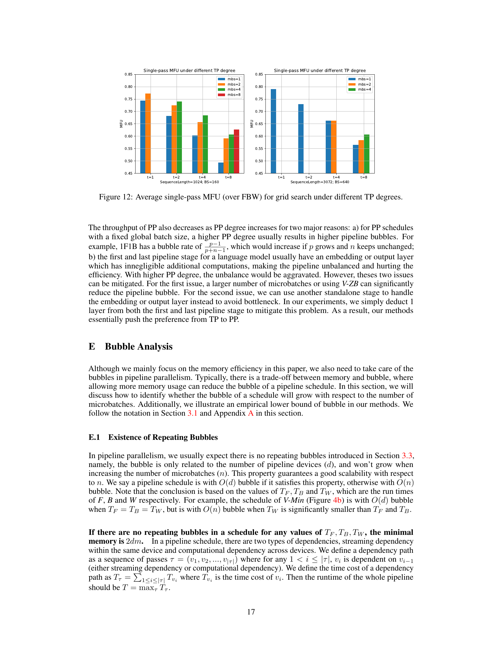
This figure shows the results of a grid search experiment that investigated the impact of different tensor parallelism (TP) degrees on the average single-pass FLOPS utilization (MFU) for forward, backward, and weight update passes (FBW). The experiment varied the microbatch size (mbs) and TP degree, demonstrating a decrease in MFU as the TP degree increased.

This figure compares different pipeline schedules, specifically V-Shape schedules (V-Min, V-Half, V-ZB) against the baseline 1F1B schedule. The comparison is made with 4 devices and 8 microbatches. The visual representation shows the sequence of forward (F), backward (B), and weight update (W) passes across the pipeline stages for each method. The goal is to illustrate how V-Shape designs lead to more efficient memory usage and reduced bubbles compared to the standard 1F1B approach. The stable phase, representing the repeating pattern in the pipeline, is highlighted to demonstrate the effect of the building block design on pipeline performance.
This figure compares different pipeline schedules (V-Min, V-Half, V-ZB, and 1F1B) under the condition of 4 devices and 8 microbatches. The schedules are represented visually using colored blocks to show the execution order of forward (F), backward (B), and weight update (W) passes for each microbatch. The stable phase of each pipeline, where the pattern repeats consistently, is clearly illustrated to show the differences in their structures and how this affects the peak memory and efficiency. The figure highlights the efficient memory management achieved by the V-shaped schedules compared to the 1F1B baseline.

This figure compares different pipeline schedules, namely 1F1B, V-Min, V-Half, and V-ZB, under the specific setting of 4 devices and 8 microbatches. It visually represents how these schedules are constructed by repeating basic building blocks. The ‘stable phases’ of the pipeline, where the pattern of the building block repeats consistently, are highlighted. This visualization helps to understand the memory efficiency and potential bubbles in each pipeline schedule.

This figure compares different pipeline schedules, specifically V-Shape schedules (V-Min, V-Half, and V-ZB) and 1F1B, under a setting of 4 devices and 8 microbatches. It visually represents the order of forward (F), backward for activations (B), and backward for weights (W) passes for each microbatch across the pipeline stages. The color-coding helps differentiate the phases. The key takeaway is that the ‘stable’ phase of each pipeline (the regularly repeating part) follows the pattern established by its building block. This visual comparison highlights the memory efficiency gains from V-Shape blocks compared to the standard 1F1B approach.

This figure shows different V-Shape building blocks with 4 devices. Each block is designed to have a balanced memory usage across devices, and it represents a sequence of forward and backward passes for a single microbatch. The white text represents the first half of the model stages, while the black text represents the second half. F, B, and W denote forward, backward (for activation gradients), and backward (for weight gradients), respectively. Each block demonstrates a different strategy for reducing peak activation memory by controlling the offsets between the passes.
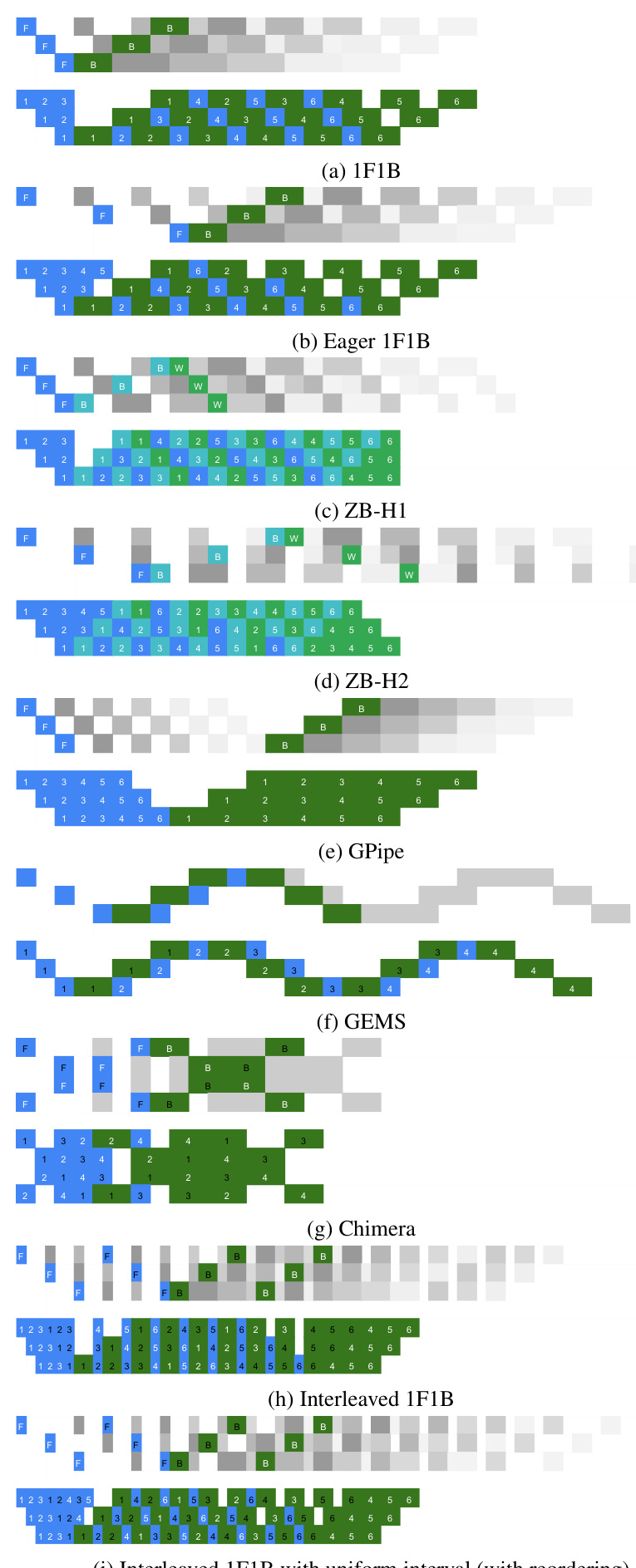
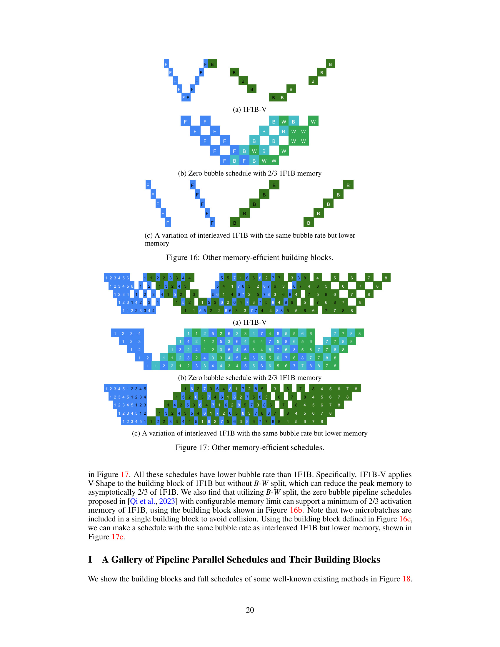
This figure illustrates the concept of building a pipeline by repeating a basic building block. It shows how a pipeline schedule (a sequence of forward and backward passes) can be constructed by repeating a smaller building block multiple times. The figure also highlights how redundant bubbles (inefficient parts of the pipeline) can be removed through a process called ‘squeezing’, resulting in a more efficient pipeline. The two examples shown are 1F1B and Eager 1F1B, showcasing different building blocks and the resulting pipelines after squeezing.
More on tables

This table presents the specifications of four different large language models (LLMs) used in the paper’s experiments. Each model is characterized by its size (in billions of parameters), the number of layers in its transformer architecture, the number of attention heads per layer, the hidden layer size, and the number of GPUs used for training. The models range in size from 9.6 billion to 98.5 billion parameters, reflecting a wide range of scales relevant to modern LLM research.
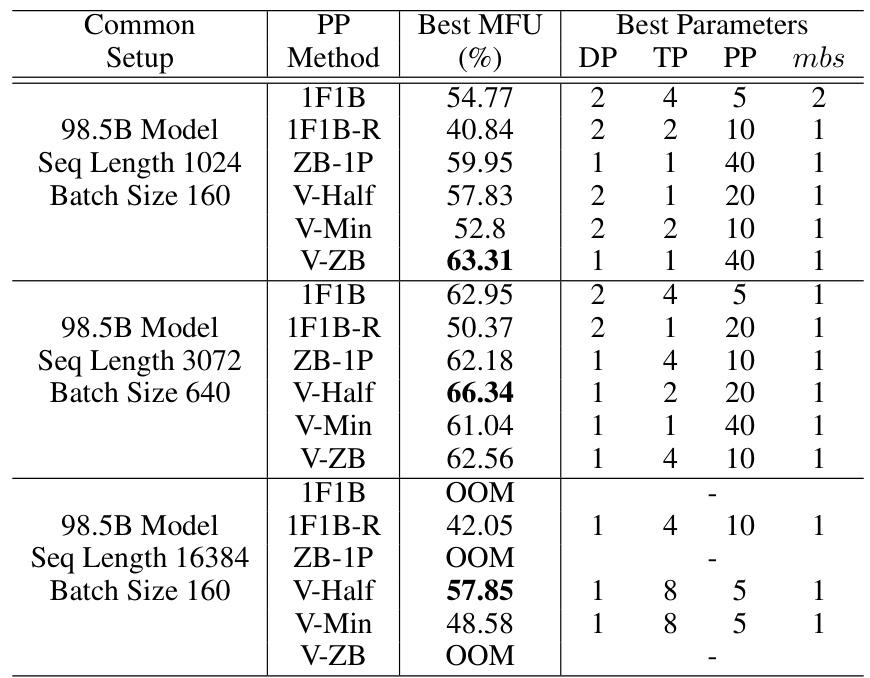
This table presents the best results obtained from grid search experiments combining V-shape schedules (V-Min, V-Half, V-ZB) with other optimization techniques (1F1B, 1F1B-R, ZB-1P) for different model sizes and sequence lengths. The table shows the best achieved MFU (model FLOPS utilization), along with the corresponding hyperparameters: DP (data parallelism), TP (tensor parallelism), PP (pipeline parallelism), and microbatch size (mbs). It demonstrates the relative performance of different scheduling approaches under various resource constraints.
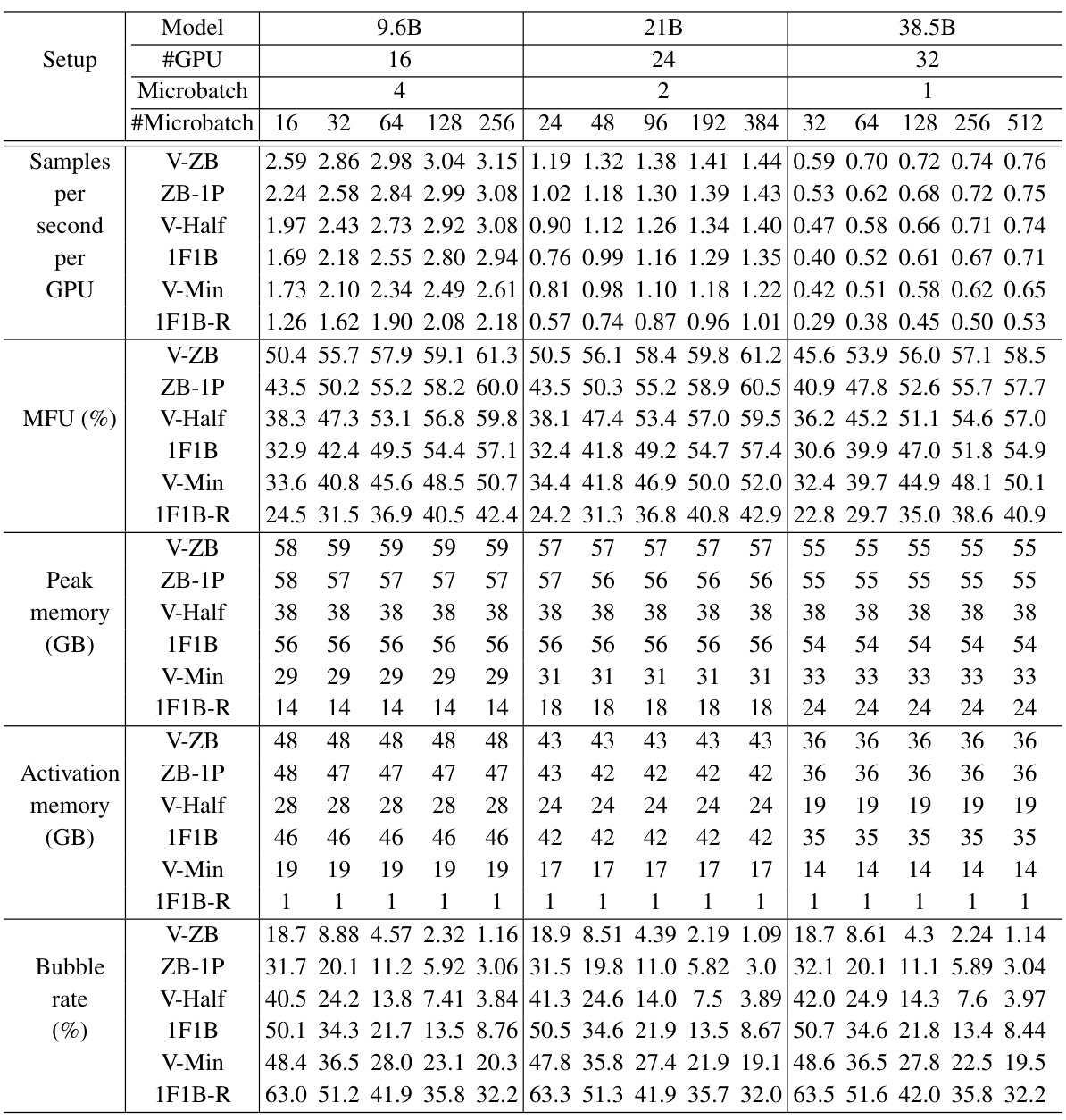
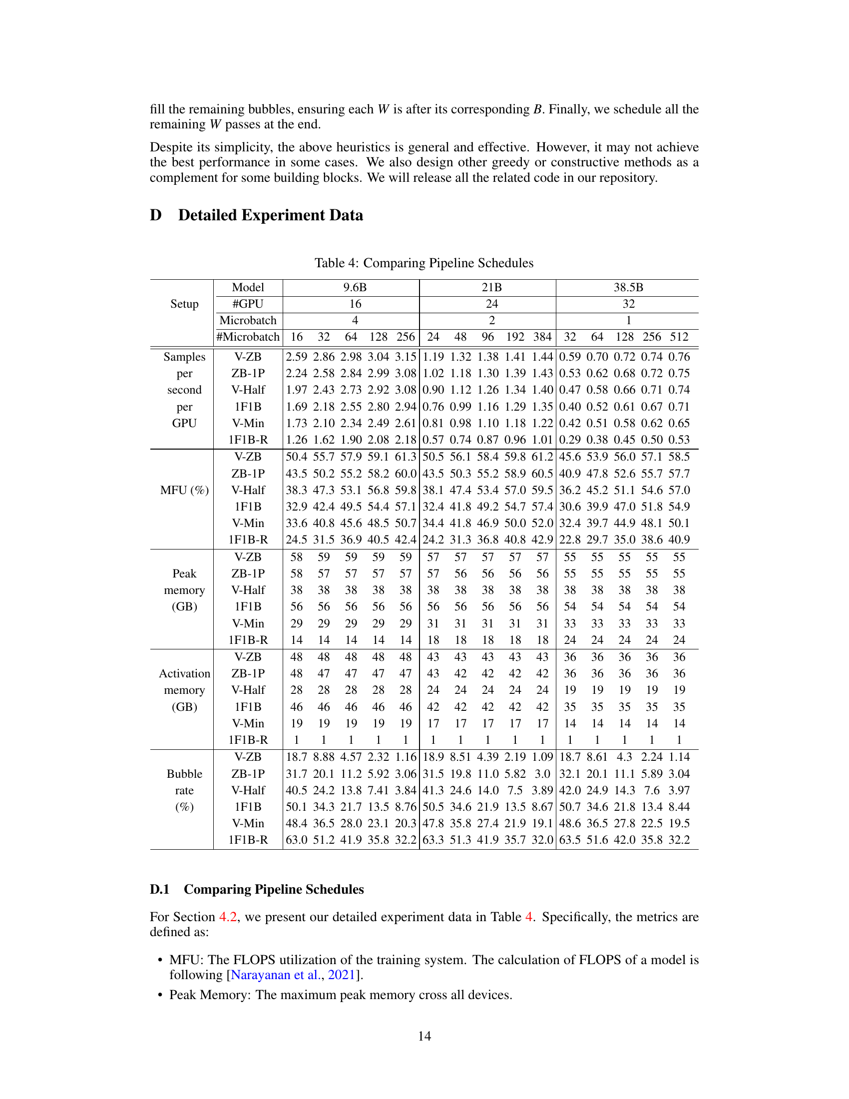
This table presents a detailed comparison of various pipeline schedules (V-ZB, ZB-1P, V-Half, 1F1B, V-Min, 1F1B-R) across three different model sizes (9.6B, 21B, 38.5B) and varying numbers of microbatches. For each schedule and model size, it shows the samples per second per GPU, the FLOPS utilization (MFU), peak memory usage, activation memory usage, and bubble rate. The data provides a quantitative comparison of the memory efficiency and throughput of different pipeline scheduling strategies.

This table shows the single-pass FLOPS utilization (MFU) for forward (F), backward (B), and weight (W) passes when the microbatch size is increased. It demonstrates how the MFU changes with different model sizes (9.6B, 21B, and 38.5B parameters) and varying microbatch sizes. The average MFU across F, B, and W passes is also provided for each configuration.

This table presents the best performance achieved by various pipeline parallel scheduling methods (1F1B, 1F1B-R, ZB-1P, V-Half, V-Min, and V-ZB) when combined with other optimization techniques such as Flash Attention, Tensor Parallelism, Sequence Parallelism, and Distributed Optimizer. The results are shown for different model sizes (98.5B) and sequence lengths (1024, 3072, 16384), highlighting the impact of each method on model parallel throughput and the optimal hyperparameter settings for each method (DP, TP, PP, and microbatch size).

This table presents the results of a grid search experiment to find the best hyperparameter settings for different pipeline parallelism schedules. It shows the Maximum FLOPS Utilization (MFU) achieved for various combinations of data parallelism (DP), tensor parallelism (TP), pipeline parallelism (PP), and microbatch size, using a sequence length of 3072 and batch size of 640. The goal was to identify the optimal configuration for each method (1F1B, 1F1B-R, ZB-1P, V-Half, V-Min, and V-ZB) in terms of MFU.

This table shows the best MFU (Million FLOPs Utilization) achieved by different pipeline parallel scheduling methods (1F1B, 1F1B-R, ZB-1P, V-Half, V-Min, V-ZB) when combined with other memory saving techniques (DP, TP, PP) for different model sizes and sequence lengths. The best parameters for each method (DP, TP, PP, and microbatch size) are also shown. It highlights the performance improvements of V-shape schedules, particularly V-Half and V-ZB, in various scenarios depending on memory pressure and model size.

This table shows the offsets used in the V-Min building block for different numbers of devices (d). The offsets are used to control the memory consumption and bubble rate of the pipeline schedule. The table shows that the offsets are designed to be different depending on whether the number of devices is a multiple of 3 or not. This ensures that there are no collisions between passes of the building blocks when they are repeated to form the pipeline. The specific values of the offsets ensure balanced peak memory across devices.

This table compares three different pipeline building blocks (1F1B, V-Min, V-Half) in terms of their peak memory consumption and number of bubbles. It shows that V-Min and V-Half significantly reduce the activation memory compared to 1F1B, while V-Half achieves near-zero bubbles. The table highlights the trade-off between memory usage and pipeline efficiency for these different approaches.
Full paper#
