Deep Graph Neural Networks via Posteriori-Sampling-based Node-Adaptative Residual Module

↗ OpenReview ↗ NeurIPS Homepage ↗ Chat

TL;DR

#

Key Takeaways

#

Why does it matter?

#

This paper is important because it addresses the over-smoothing problem in deep Graph Neural Networks (GNNs), a critical issue hindering their performance. The proposed PSNR module offers a novel, efficient solution, improving GNN scalability and accuracy, especially when dealing with incomplete data. This opens avenues for developing more robust and effective GNNs for various applications.

Visual Insights

#

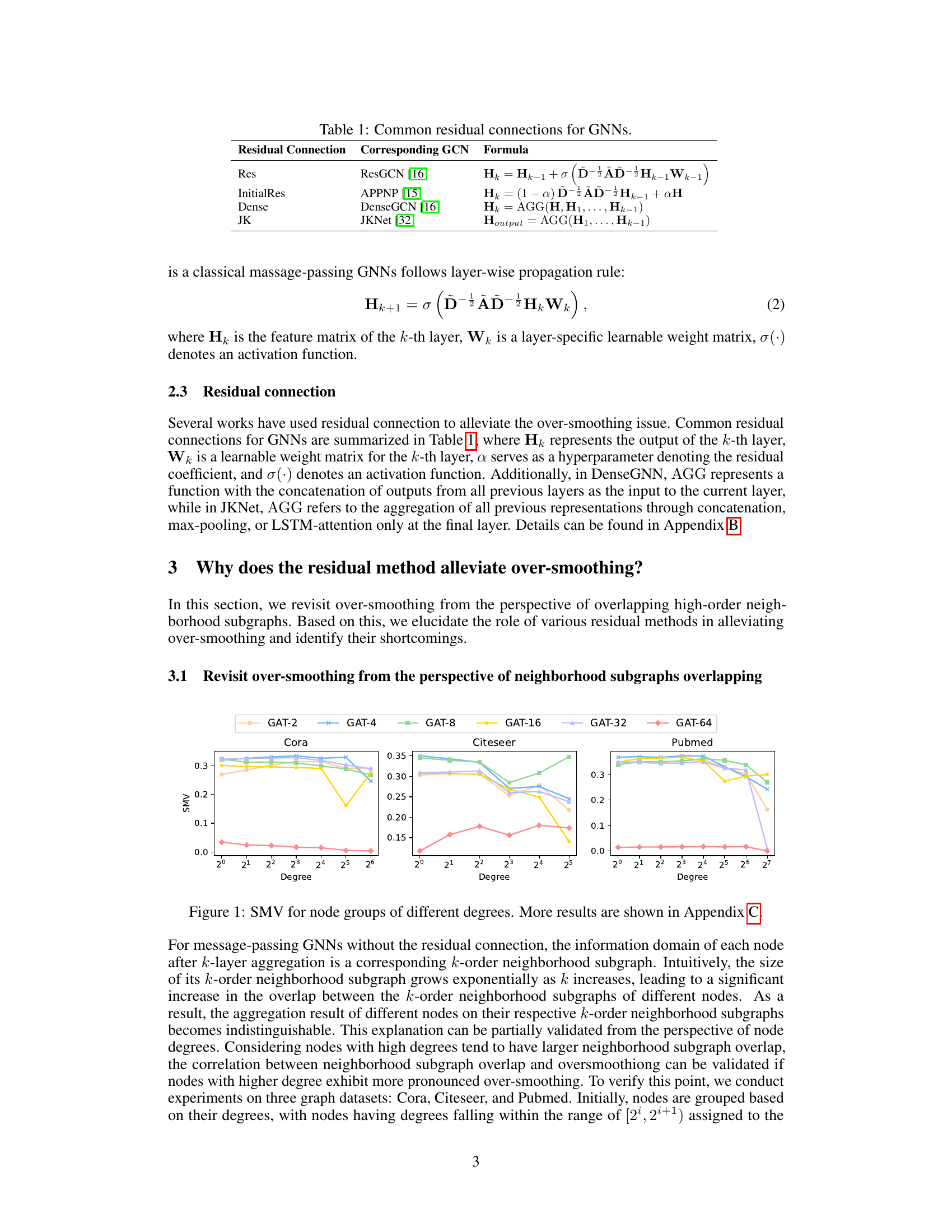
This figure displays the Smoothness Metric Value (SMV) for nodes grouped by their degrees, using the GAT model with varying numbers of layers (2, 4, 8, 16, 32, 64). The SMV measures how similar node representations become as the number of layers increase in a GNN. The results show the relationship between node degree and over-smoothing. Nodes with higher degrees tend to show higher SMV values, indicating higher over-smoothing, as their neighborhood subgraphs have more overlap. This observation is used to support the paper’s argument on over-smoothing from the perspective of overlapping neighborhood subgraphs. Appendix C contains additional results for other models and datasets.

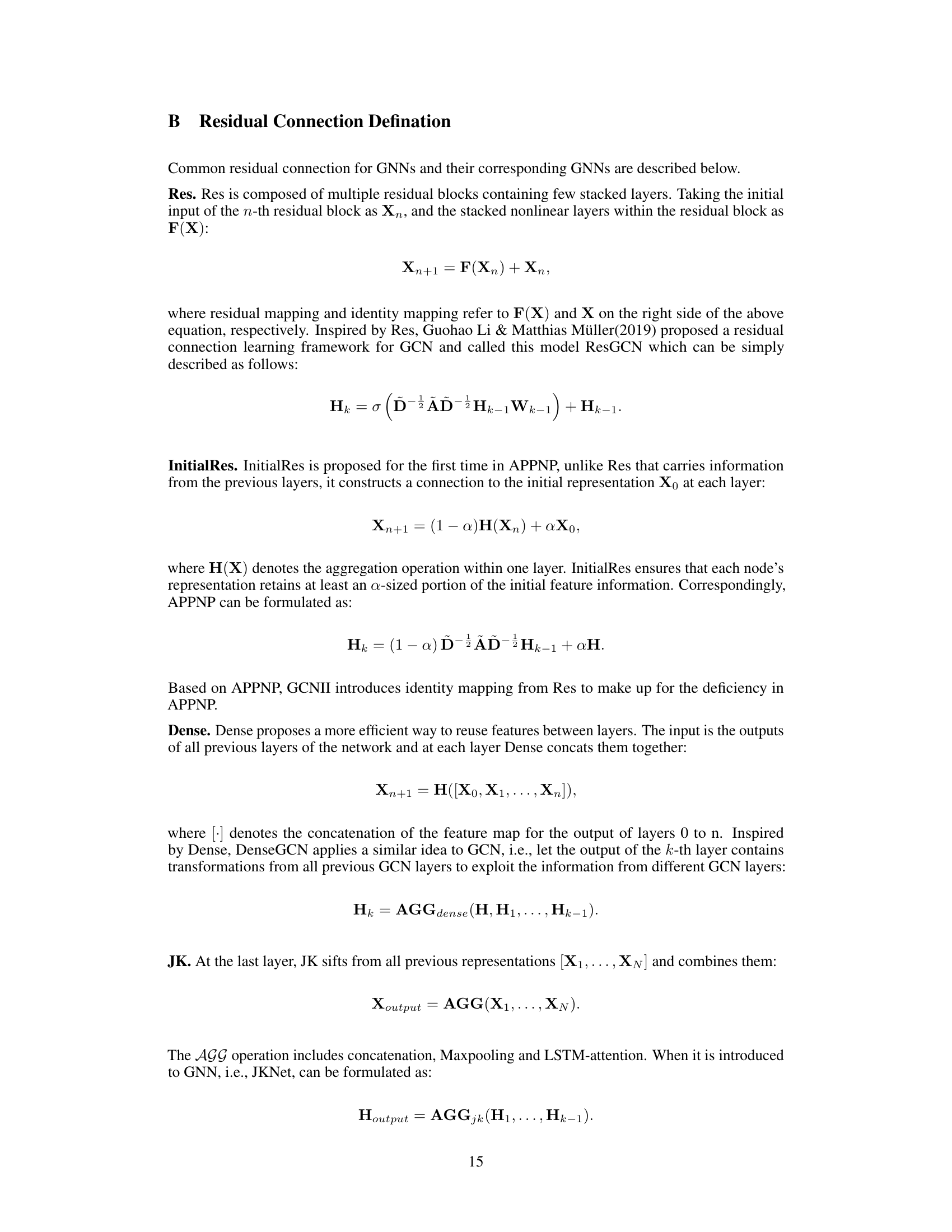
This table summarizes common residual connections used in Graph Neural Networks (GNNs) to alleviate the over-smoothing issue. It lists four types of residual connections (Res, InitialRes, Dense, JK) along with their corresponding GCN formulas. Each formula shows how the output of the k-th layer (Hk) is calculated, incorporating residual connections with different aggregation strategies of previous layers’ outputs.

In-depth insights

#

Over-smoothing Revisited

#

Over-smoothing, a phenomenon where node representations in deep Graph Neural Networks (GNNs) become indistinguishable, is revisited. The core issue is identified as overlapping high-order neighborhood subgraphs, leading to information redundancy and hindering the model’s ability to learn distinctive features. This perspective helps clarify how residual methods, by integrating multiple orders of neighborhood information, mitigate over-smoothing. However, existing residual methods are criticized for lacking node adaptability and causing a severe loss of high-order subgraph information. A novel approach is proposed to address these limitations, suggesting a more nuanced understanding and improved solutions for tackling over-smoothing in GNNs.

PSNR Module

#

The PSNR (Posterior-Sampling-based Node-Adaptive Residual) Module is a novel approach to address over-smoothing in deep Graph Neural Networks (GNNs). It leverages a graph encoder to learn node-specific residual coefficients, avoiding the limitations of previous methods that use fixed coefficients. This node-adaptability allows for finer-grained control over the information aggregation process and prevents the loss of high-order neighborhood subgraph information that often plagues deep GNNs. The PSNR module introduces randomness during both training and testing, improving generalization and mitigating oversmoothing. By dynamically adjusting the residual connections based on the posterior distribution of the coefficients, PSNR allows GNNs to effectively model long-range dependencies and significantly improves performance, especially in cases of missing features where deep networks are essential.

Adaptive Residuals

#

The concept of “Adaptive Residuals” in deep learning models, particularly within the context of Graph Neural Networks (GNNs), presents a powerful approach to mitigate the over-smoothing problem. Adaptive residuals go beyond the traditional static residual connections by dynamically adjusting the residual components based on node-specific characteristics or layer-wise needs. This adaptability is crucial because nodes in a graph exhibit varying degrees of information richness and connectivity, requiring a more nuanced approach than a uniform residual across all nodes. By learning these adaptive weights, the model can selectively integrate information from different layers or neighborhood aggregations, preventing information loss and maintaining node identity at deeper layers. This approach is especially valuable for scenarios with missing data or when dealing with graphs with complex topological structures. The challenge lies in effectively learning these adaptive components without introducing excessive computational overhead, hence the need for efficient learning mechanisms, such as those based on posterior sampling or graph attention networks. Overall, adaptive residuals represent a significant advancement in GNN design, offering a pathway towards building deeper and more robust models capable of handling intricate graph patterns and incomplete data. The use of a graph encoder within the adaptive residual module also signifies a powerful approach to integrate node features and graph structure for improved performance.

Deep GNNs

#

Deep Graph Neural Networks (GNNs) hold immense potential but face challenges as depth increases. Over-smoothing, where node representations become indistinguishable, significantly hinders performance. Many approaches, including various residual methods, attempt to mitigate this. Residual connections aim to preserve initial information and integrate multi-order neighborhood subgraphs, counteracting the homogenizing effect of repeated aggregation. However, existing methods often lack node-adaptability, uniformly applying residual connections regardless of node characteristics and potentially losing information. A novel, adaptive residual module is needed to address these shortcomings, enabling more effective learning from graph structures, even at substantial depths.

Scalability & Limits

#

A crucial aspect of any machine learning model is its scalability and inherent limitations. Scalability refers to the model’s ability to handle increasing amounts of data and computational demands efficiently. For graph neural networks (GNNs), scalability is challenged by the complexity of graph operations, especially as graph size and depth grow. Memory constraints become a significant bottleneck for larger graphs due to the storage of node embeddings and adjacency matrices. Computational costs rise with increasing graph size and depth, limiting the applicability of GNNs to very large-scale datasets. Addressing these challenges often requires innovative techniques like graph sampling or efficient aggregation methods. Model limitations arise from the inherent inductive biases of GNNs. Over-smoothing, where node representations become indistinguishable, can severely hamper performance in deep GNNs. The choice of architecture, message-passing scheme, and aggregation functions all significantly impact performance and scalability. Overfitting is also a concern, particularly with deep architectures and limited data. Therefore, understanding the trade-offs between model capacity, computational resources, and data requirements is vital when designing and applying GNNs to real-world problems. Careful consideration of these factors is crucial for successful deployment at scale. Future research should focus on developing more efficient algorithms and architectures that mitigate scalability issues and improve the robustness and generalizability of deep GNNs.

More visual insights

#

More on figures

This figure shows the architecture of the Posteriori-Sampling-based Node-Adaptive Residual module (PSNR). The PSNR module takes the output of a previous GNN layer (Hk-1) as input. A GNN layer processes this input to produce H’k-1. These are then fed into an encoder along with the adjacency matrix (A) and positional embedding (LayerEmb(k)) to obtain the posterior distribution of the residual coefficients (ηk). This distribution is then sampled to obtain node-adaptive residual coefficients which are then used to compute the final output (Hk) via a residual connection with the initial input.

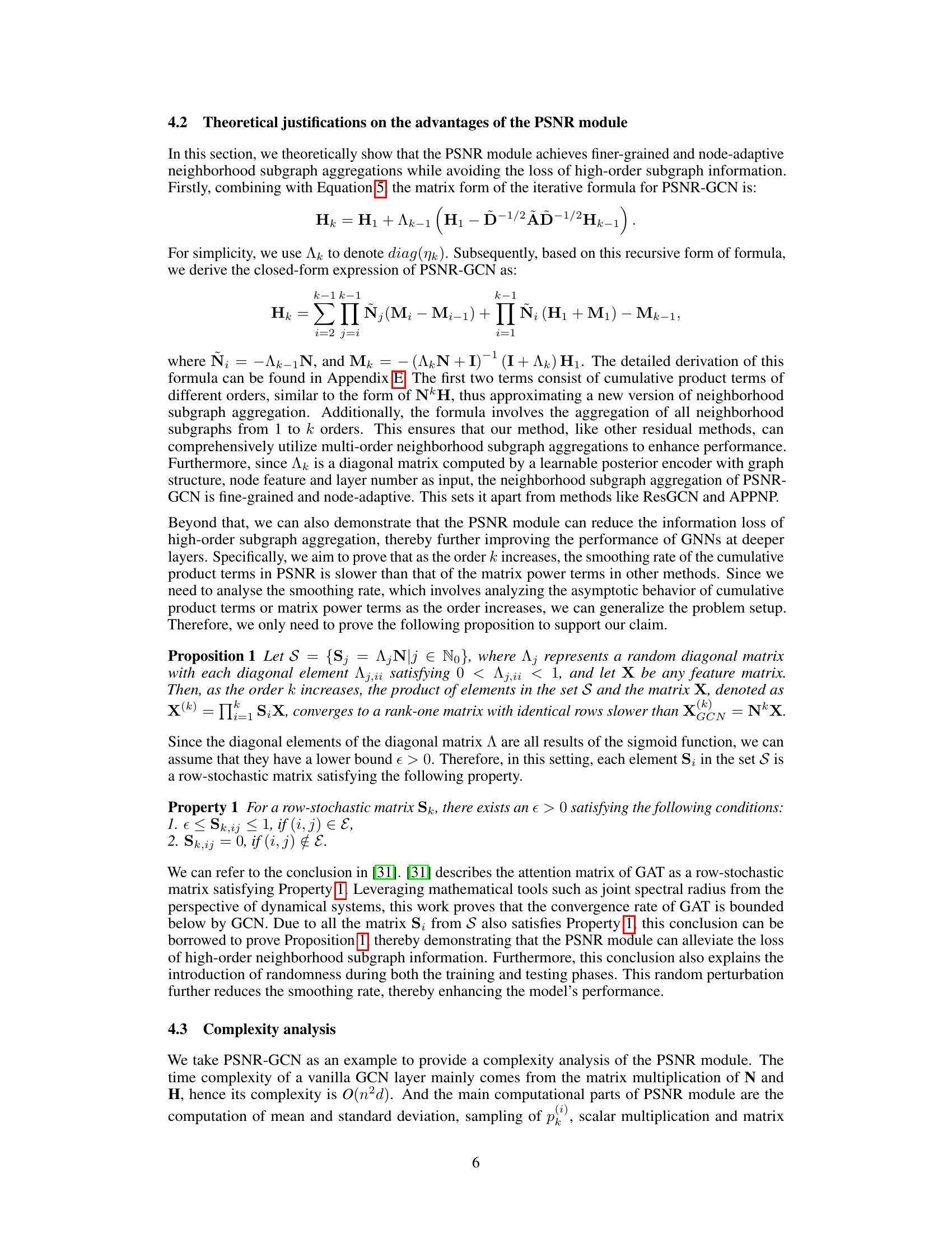
The figure shows the effectiveness of different residual methods in mitigating over-smoothing in deep GNNs. The x-axis represents the number of layers and the y-axis represents the accuracy. The results demonstrate that the PSNR module consistently outperforms other methods in maintaining stable performance even at significantly deeper layers (64 layers). This is because PSNR effectively mitigates the loss of high-order neighborhood subgraph information, which is crucial for maintaining performance in deep GNNs.

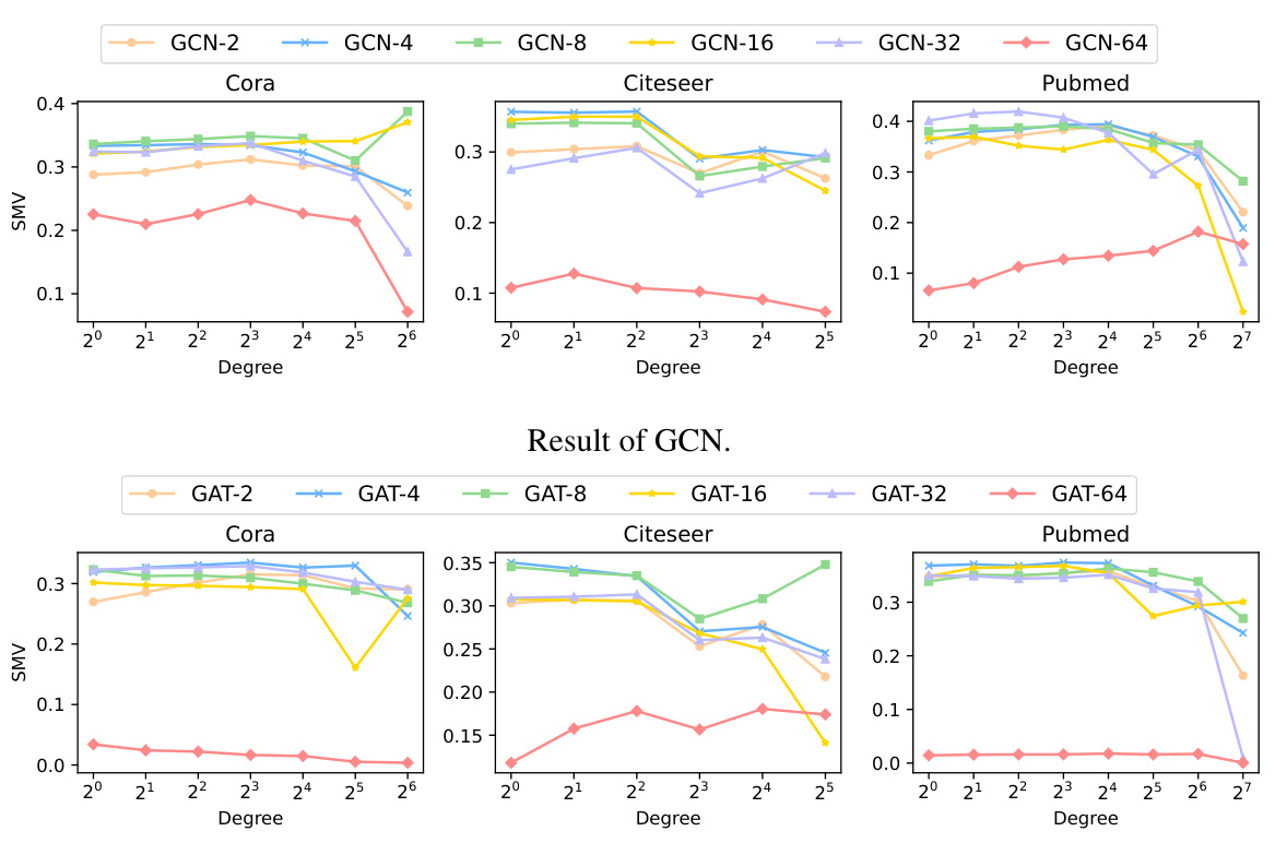
This figure shows the Smoothness Metric Value (SMV) for different node degree groups across various layers of GCN and GAT models. Higher SMV indicates more over-smoothing. It visually demonstrates that nodes with higher degrees exhibit more over-smoothing, supporting the paper’s claim that over-smoothing is related to overlapping high-order neighborhood subgraphs.

More on tables

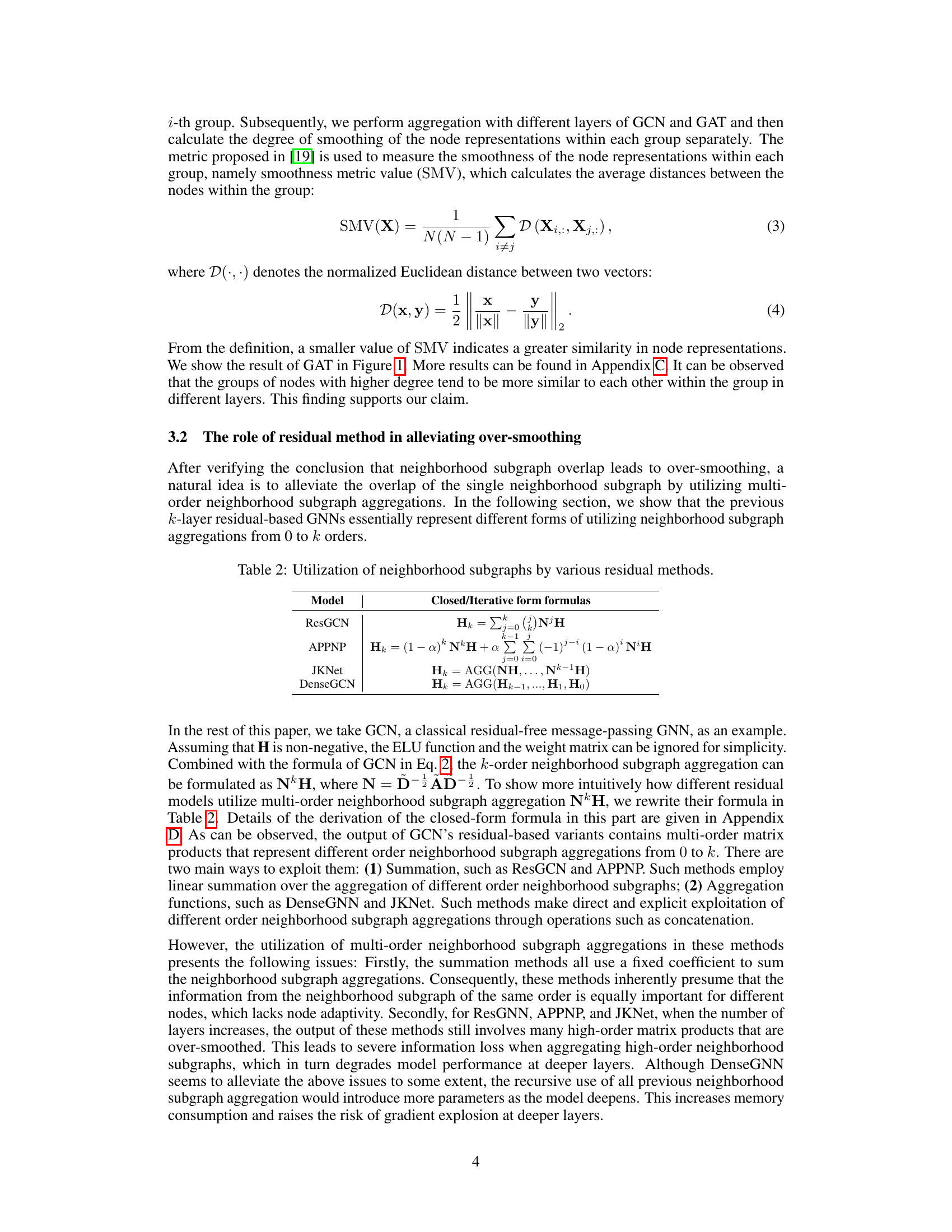
This table shows how different residual methods utilize neighborhood subgraphs from order 0 to k. ResGCN and APPNP use summation, while DenseGCN and JKNet use aggregation functions to combine subgraph information. The formulas demonstrate how each method incorporates multiple orders of neighborhood information.

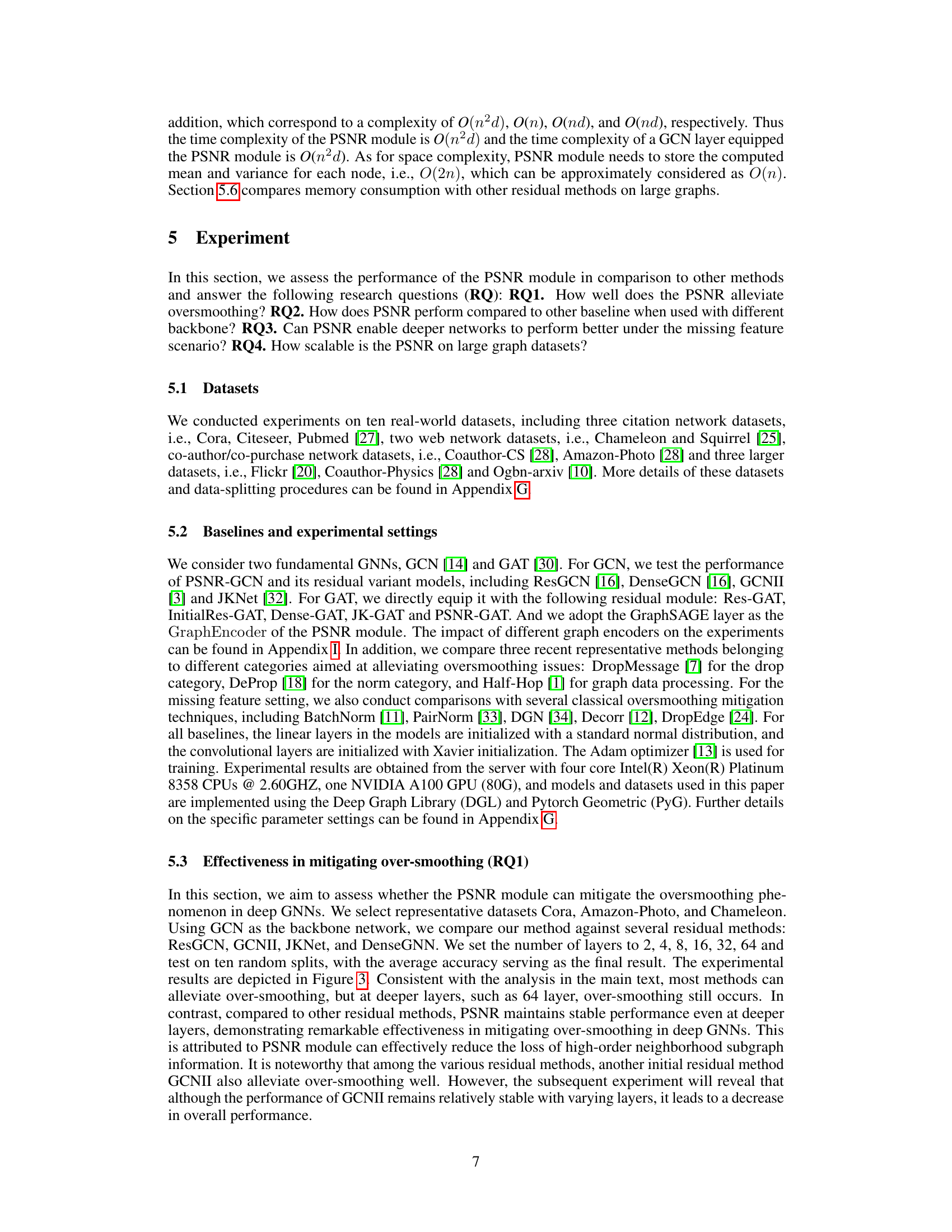
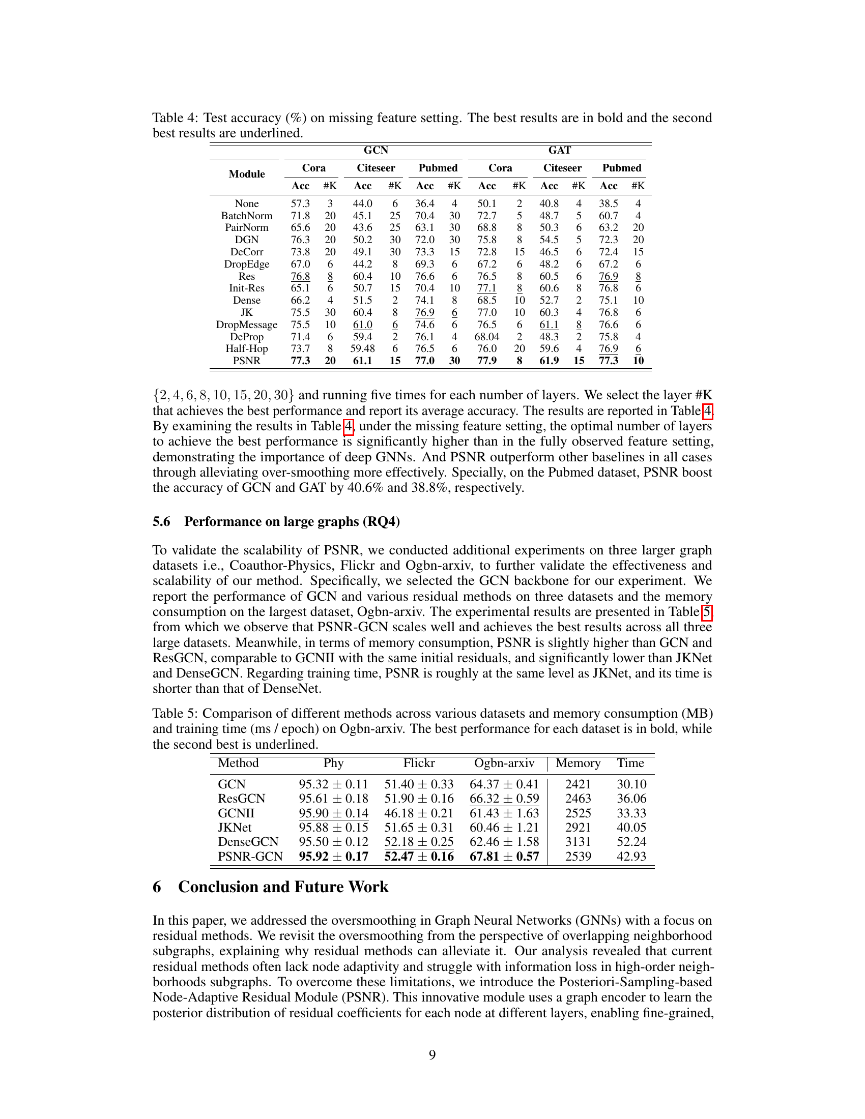
This table presents a comparison of classification accuracy across various GNN models (GCN and GAT, with several residual connection methods) on ten real-world datasets. The accuracy is shown for each model on each dataset, with the best performing model for each dataset highlighted in bold and the second-best underlined. This allows for a direct performance comparison between different GNN architectures and the impact of different residual methods.

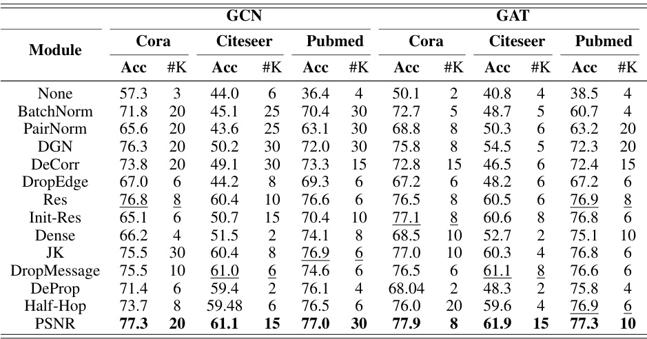
This table presents a comparison of the classification accuracy achieved by various GNN models (GCN and GAT with different residual connections) across ten real-world datasets. The accuracy is reported as a percentage, averaged over multiple runs, with error bars omitted. The best and second-best performances for each dataset are highlighted in bold and underlined, respectively. The table allows for a comparison of different residual connection techniques to mitigate over-smoothing, with performance assessed at varying numbers of layers.

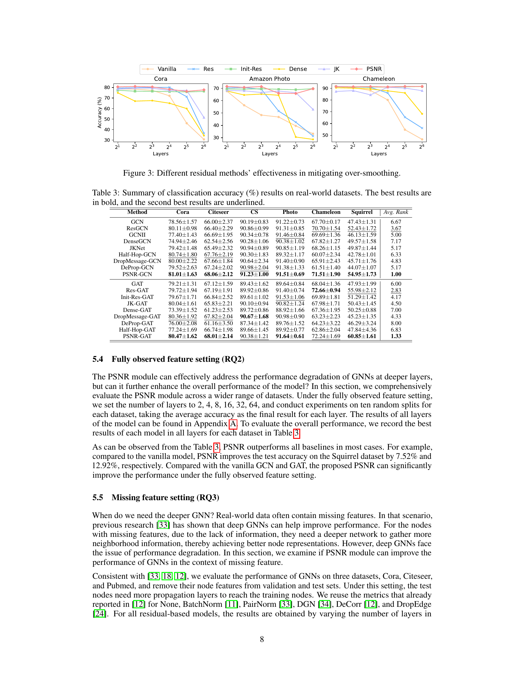
This table compares the performance of various GNN models (GCN, ResGCN, GCNII, JKNet, DenseGCN, and PSNR-GCN) on three large graph datasets (Coauthor-Physics, Flickr, and Ogbn-arxiv). The metrics used are accuracy and memory consumption (in MB) and training time (in ms per epoch) on the largest dataset (Ogbn-arxiv). The best performing model for each dataset is highlighted in bold, with the second-best underlined. This table demonstrates the scalability and performance of PSNR-GCN compared to other methods.

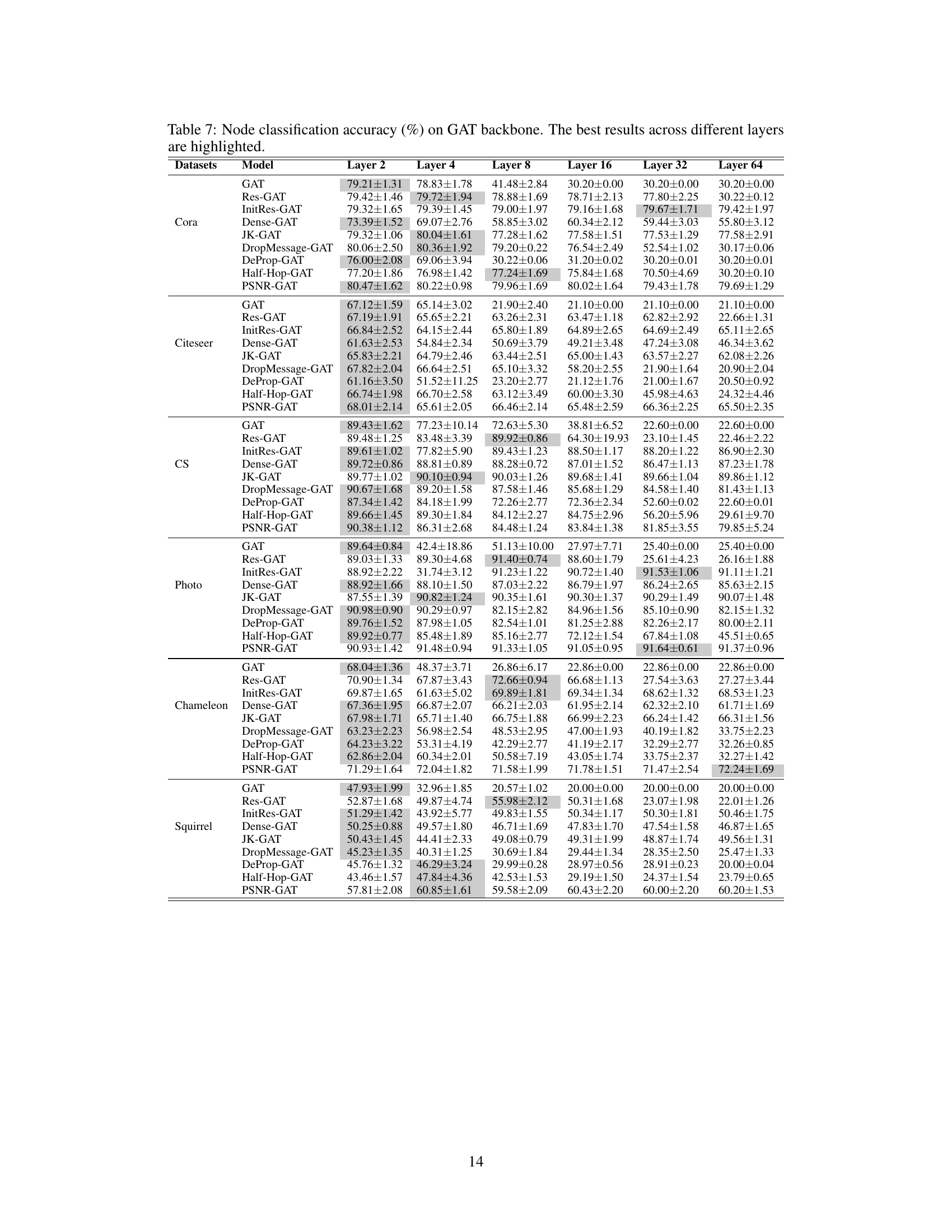
This table presents the node classification accuracy achieved by various GCN models (GCN, ResGCN, GCNII, DenseGCN, JKNet, DropMessage-GCN, Half-Hop-GCN, DeProp-GCN, and PSNR-GCN) across six different layer depths (2, 4, 8, 16, 32, and 64) on various datasets (Cora, Citeseer, CS, Photo, Chameleon, and Squirrel). The best accuracy for each dataset at each layer depth is highlighted to demonstrate the comparative performance of these models in mitigating oversmoothing at varying network depths.

This table presents the node classification accuracy achieved by different GNN models (GCN, ResGCN, GCNII, DenseGCN, JKNet, DropMessage-GCN, Half-Hop-GCN, DeProp-GCN, and PSNR-GCN) on various datasets (Cora, Citeseer, CS, Photo, Chameleon, Squirrel). The accuracy is shown for different numbers of layers (2, 4, 8, 16, 32, 64) in the GNN architecture. The best accuracy for each dataset across all layer numbers is highlighted, demonstrating the performance of each model at varying depths and its effectiveness in mitigating over-smoothing.

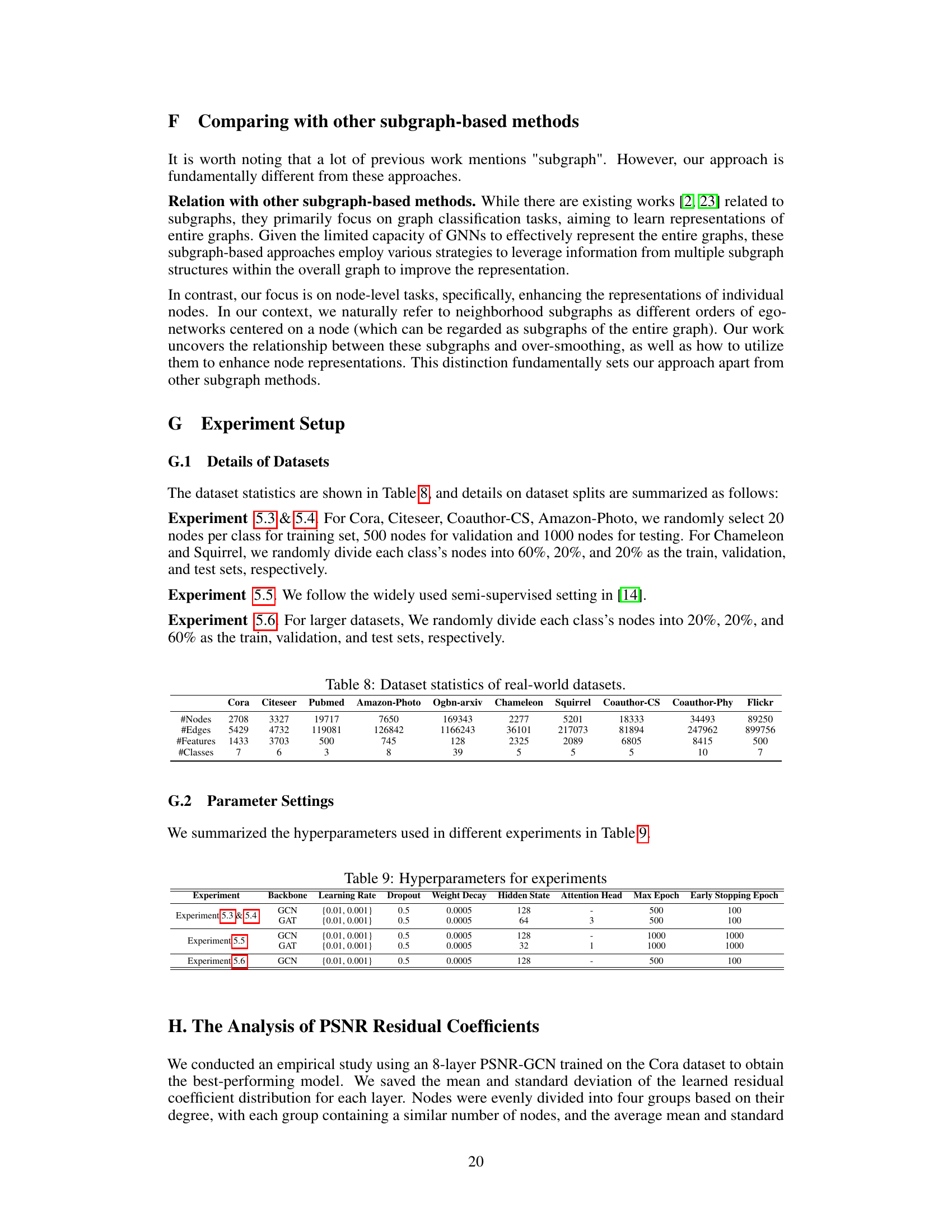
This table presents the key statistics for ten real-world datasets used in the paper’s experiments. The datasets are diverse, encompassing citation networks (Cora, Citeseer, Pubmed), web networks (Chameleon, Squirrel), co-authorship/co-purchase networks (Coauthor-CS, Amazon-Photo, Coauthor-Physics), and a large-scale dataset from Ogbn (Ogbn-arxiv). For each dataset, the number of nodes, edges, features, and classes are provided, showcasing the variability in size and complexity of the graph data used.

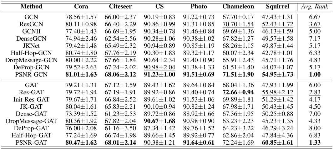
This table presents the classification accuracy results of various GNN models (GCN and GAT with different residual connection methods including ResGCN, GCNII, DenseGCN, JKNet, PSNR, Half-Hop, DropMessage, DeProp) on ten real-world datasets (Cora, Citeseer, CS, Photo, Chameleon, Squirrel, etc.). The table shows the average accuracy and rank for each model on each dataset. The best and second-best performing models are highlighted in bold and underlined respectively. This allows for a comparison of the performance of different GNN models across various datasets. The average rank of each model across all datasets is also shown.

This table presents a comparison of the classification accuracy achieved by various GNN models (including the proposed PSNR model) on ten different real-world datasets. The accuracy is shown for each model on each dataset, and the best and second-best results are highlighted for easy comparison. The table allows readers to quickly assess the relative performance of the different models across different datasets.

This table presents the performance comparison of different graph encoders (GCN, GAT, and SAGE) on the node classification task using the PSNR module with two layers. The results are shown for six different datasets: Cora, Citeseer, CS, Photo, Chameleon, and Squirrel. The table allows readers to assess the impact of different encoder choices on the overall performance of the proposed PSNR module.

This table presents the classification accuracy results of different GNN models (GCN and GAT with various residual methods including PSNR) on ten real-world datasets. The best and second-best accuracies for each dataset are highlighted in bold and underlined, respectively. The average rank of each model across all datasets is also given to provide a comprehensive comparison. This helps assess the overall performance of the proposed PSNR method compared to other existing methods for node classification in various graph scenarios.

Full paper

#