↗ OpenReview ↗ NeurIPS Homepage ↗ Chat
TL;DR#
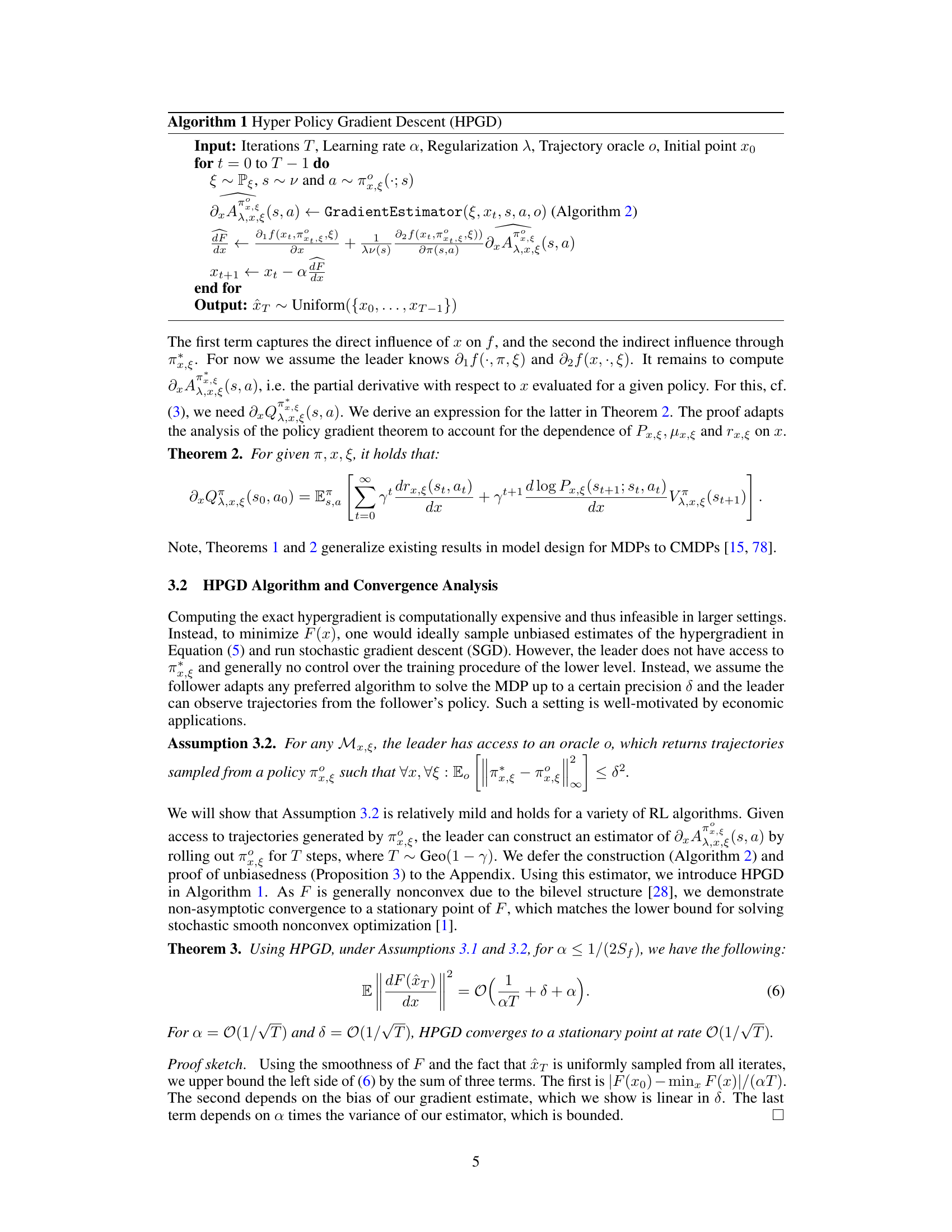
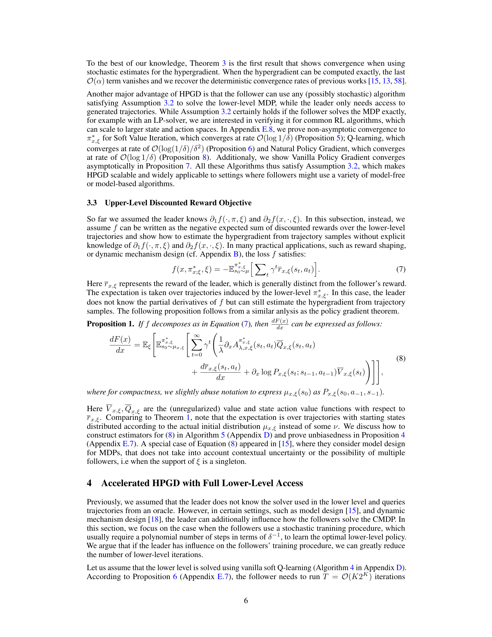
Many real-world problems involve hierarchical decision-making where a leader’s actions influence followers’ responses within a dynamic environment. Existing approaches often struggle with such complex scenarios due to assumptions on follower algorithm and the high computational cost of computing the hypergradient. This paper presents a new approach, Contextual Bilevel Reinforcement Learning (CB-RL), which models these settings as a contextual Markov Decision Process (CMDP) at the follower level and utilizes a stochastic bilevel optimization approach.
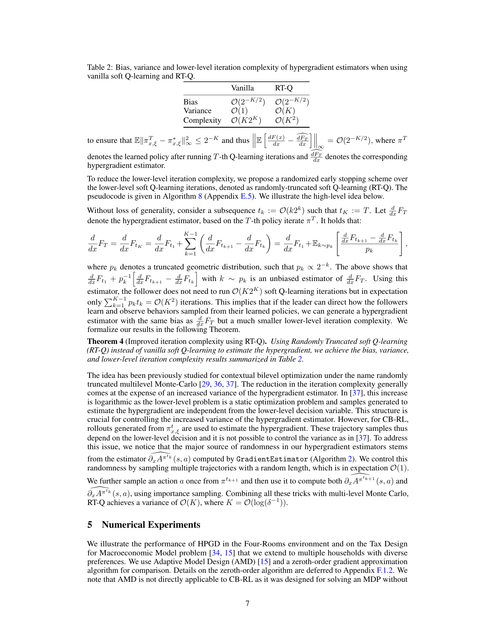
The proposed solution, stochastic Hyper Policy Gradient Descent (HPGD), directly addresses the limitations of previous methods. It only needs to observe follower trajectories instead of the full gradient, enabling the use of any follower training procedure, making it adaptable to various real-world situations. HPGD shows convergence and is empirically demonstrated for reward shaping and tax design, showcasing its effectiveness in handling complex, large-scale problems where deterministic algorithms struggle.
Key Takeaways#
Why does it matter?#
This paper is crucial for researchers working on incentive alignment and multi-agent reinforcement learning (MARL). It introduces a novel framework and algorithm, addressing the limitations of existing bilevel RL approaches. Its impact extends to various fields like RLHF, tax design, and mechanism design, offering scalable solutions for complex real-world problems. The use of stochastic hypergradient estimates makes it widely applicable, opening avenues for future research in handling multiple followers and side information within hierarchical decision-making systems.
Visual Insights#
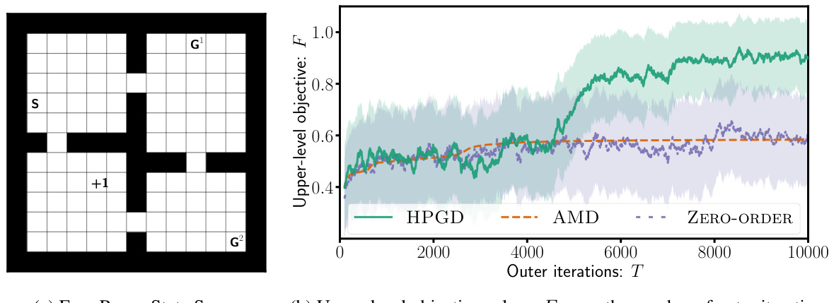
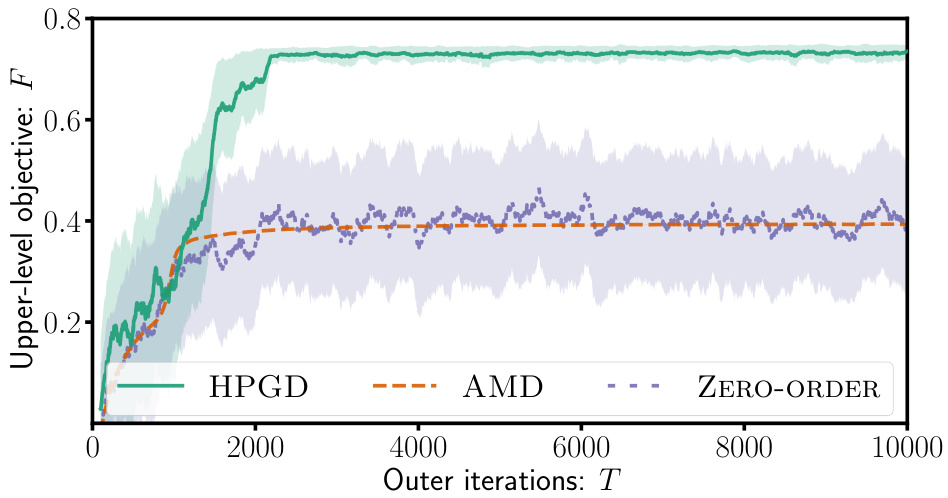
This figure contains two subfigures. The left subfigure shows a diagram of the Four-Rooms environment used in the experiment. The right subfigure shows a plot of the upper-level objective function F (y-axis) versus the number of outer iterations T (x-axis). The plot compares the performance of three algorithms: HPGD, AMD, and Zero-Order. The results indicate that HPGD outperforms the other two algorithms, particularly by avoiding local optima.
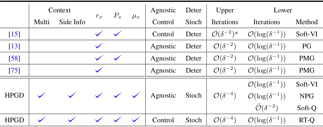
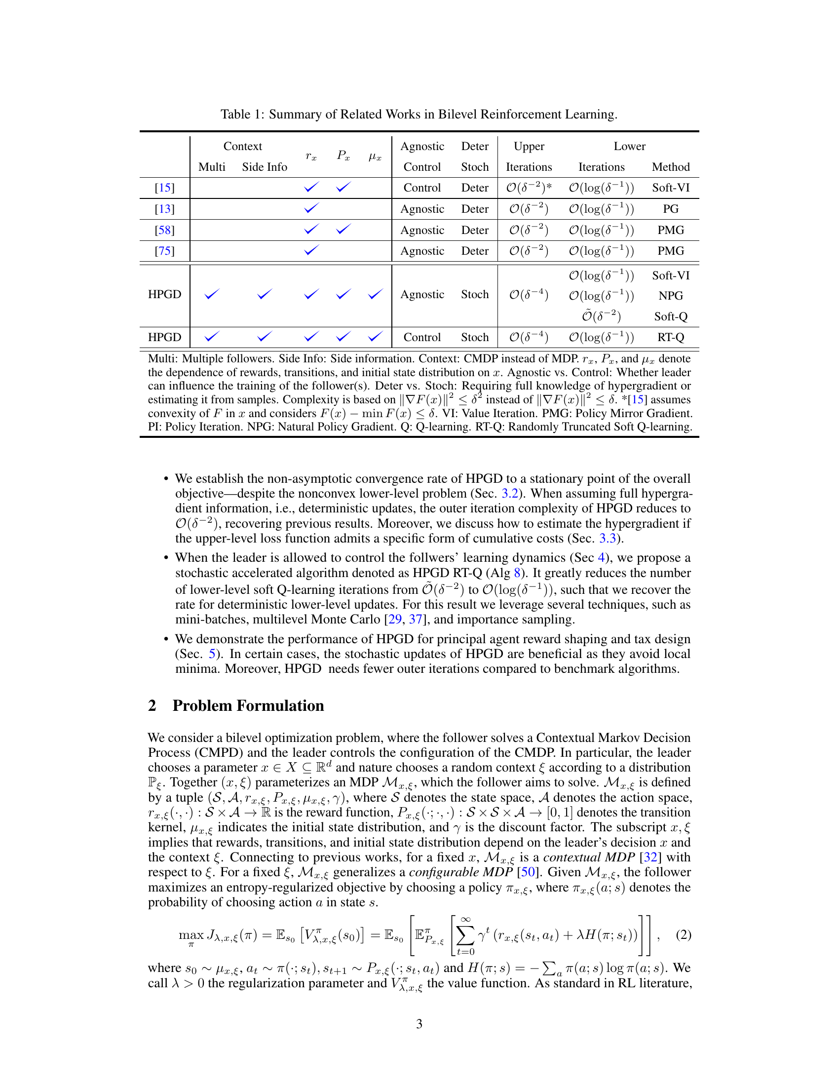
The table summarizes and compares several existing works in bilevel reinforcement learning. It highlights key differences across these papers, focusing on whether the leader’s algorithm is agnostic to the follower’s algorithm, whether the updates are deterministic or stochastic, the iteration complexity for the upper and lower levels, and the specific algorithm used. The table also shows whether the methods considered multiple followers, contextual information, and side information.
In-depth insights#
CB-RL Framework#
The Contextual Bilevel Reinforcement Learning (CB-RL) framework offers a novel approach to hierarchical reinforcement learning problems where environmental context significantly influences optimal policies. It models a Stackelberg game, with a leader (upper level) configuring a contextual Markov Decision Process (CMDP) and followers (lower level) responding optimally within that context. This approach is particularly valuable in scenarios with exogenous events impacting decision-making. The leader’s objective is to optimize an overall goal by anticipating the followers’ responses to contextual information. The follower’s objective is to maximize their individual reward within the given CMDP. A key strength lies in its agnostic treatment of follower algorithms; the framework doesn’t prescribe specific training methods, enhancing its flexibility and applicability to diverse real-world situations. The CB-RL framework’s capacity to handle multiple followers and integrate side information also distinguishes it from previous hierarchical RL models. This makes it particularly suitable for applications like reward shaping, tax design, and mechanism design, where the leader’s actions impact the environment’s configuration and subsequently influence the agents’ choices.
HPGD Algorithm#
The Hyper Policy Gradient Descent (HPGD) algorithm is a novel approach to solve the Contextual Bilevel Reinforcement Learning (CB-RL) problem. It cleverly addresses the challenge of hypergradient estimation by relying on stochastic estimates derived from follower trajectories, rather than exact calculations. This agnostic approach to follower training methods allows flexibility and scalability in real-world applications. The algorithm’s convergence is theoretically proven, demonstrating its ability to reach a stationary point. Furthermore, HPGD shows empirical effectiveness, particularly in situations where stochasticity helps escape local optima, such as in reward shaping and tax design problems, showcasing its practical applicability.
Convergence Rate#
The convergence rate analysis is crucial for evaluating the efficiency and practicality of any iterative algorithm. In this context, establishing a non-asymptotic convergence rate is particularly valuable, as it provides concrete bounds on the number of iterations required to reach a desired level of accuracy, unlike asymptotic rates which only describe the long-term behavior. The paper demonstrates a convergence rate of O(1/√T) for the stochastic HPGD algorithm under specific assumptions about the smoothness and Lipschitz continuity of the objective function and an inexact oracle providing lower-level trajectory data. This indicates that the algorithm’s performance is guaranteed to improve as the number of iterations increases, but at a relatively slow rate. The choice of step size (α) is shown to influence the convergence rate significantly, with a recommended choice depending on the smoothness constant (Sf). Furthermore, the analysis reveals the impact of the lower-level solver’s inexactness (δ), suggesting that a more accurate lower-level solution translates to faster convergence at the upper level. Ultimately, these findings are essential to assess algorithm’s scalability and applicability in practical settings.
Empirical Results#
An effective ‘Empirical Results’ section would meticulously detail experimental setups, including algorithms, hyperparameters (and their selection rationale), evaluation metrics, and baselines. Crucially, it should present results clearly and concisely, using appropriate visualizations (e.g., graphs, tables) to showcase key findings. Statistical significance should be rigorously addressed through error bars or hypothesis testing to ensure that observed effects aren’t due to random chance. The discussion should go beyond simply reporting numbers and delve into interpreting the results, comparing performance across different settings and baselines, and connecting back to the paper’s core claims. Limitations of the experimental design and potential biases should be acknowledged to ensure the overall analysis is balanced and robust. Finally, a discussion on resource usage in terms of computing time and power is highly recommended for reproducibility.
Future of CB-RL#
The future of Contextual Bilevel Reinforcement Learning (CB-RL) is promising, given its potential to model complex real-world scenarios. Further research should focus on improving the scalability of algorithms, such as developing more efficient hypergradient estimation techniques that reduce reliance on computationally expensive exact methods. Addressing the challenge of non-convexity in the lower-level optimization problem is also crucial for ensuring reliable and efficient convergence. Exploration of advanced architectures, including deep learning methods tailored for the bilevel structure, could enhance CB-RL’s ability to tackle high-dimensional and complex problems. Developing more robust methods for handling uncertainty and partial observability in the contextual information will significantly expand its applicability. Finally, exploring applications beyond the examples presented (RLHF, tax design, reward shaping) is vital to establish the broader impact of this framework. The ability of CB-RL to address real-world scenarios where leaders interact with heterogeneous followers in complex environments makes it a particularly relevant area of future research.
More visual insights#
More on figures

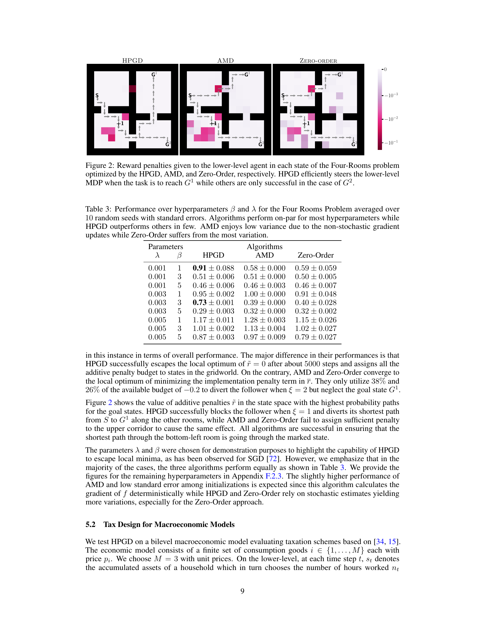
This figure shows the reward penalties assigned to each state by three different algorithms: HPGD, AMD, and Zero-Order, in the Four-Rooms environment. The goal is to guide the lower-level agent to a specific target state (+1). HPGD effectively achieves this goal for G¹, whereas AMD and Zero-Order only succeed for G². The visualization uses a color map to represent penalty magnitude, showing the strategy used by each algorithm.

This figure shows the performance of the HPGD and Zero-Order algorithms on the Tax Design problem. The left panel displays the upper-level objective values over the number of outer iterations. The right panel shows the tax rates (income tax and VAT rates for three goods) over the outer iterations. The results demonstrate that HPGD quickly learns optimal tax policies that distinguish VAT rates according to consumer preferences. Zero-Order, in contrast, takes significantly more iterations to achieve a similar level of performance.

The figure consists of two subfigures. The left subfigure shows the state space of the Four-Rooms environment, which is a grid-world with four rooms and a goal in each room. The start state (S) is in the top-left corner, and there are two goal states (G¹ and G²) located in different rooms. The +1 symbol indicates a target cell. The right subfigure shows the performance of three different algorithms (HPGD, AMD, and Zero-Order) in terms of the upper-level objective value (F) as a function of the number of outer iterations (T). The HPGD algorithm consistently performs better than the other two, demonstrating its ability to escape local optima and achieve higher performance.
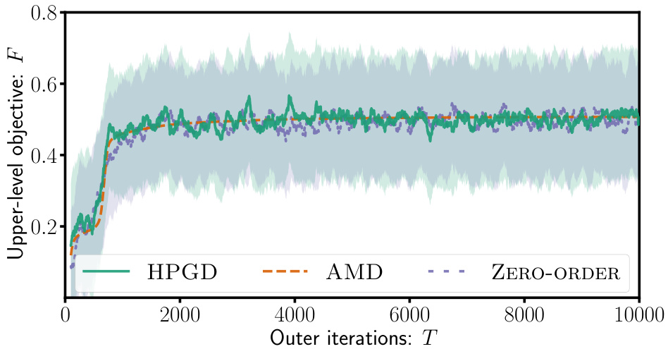
The figure shows the results of experiments conducted using the Four-Rooms environment. The left panel depicts the state space of the environment, highlighting the start state (S), two goal states (G¹ and G²), and a target cell (+1) that the upper-level algorithm aims to influence the lower-level agent to reach. The right panel presents a comparison of the performance of three different algorithms: HPGD, AMD, and a Zero-Order method, demonstrating HPGD’s superior ability to reach higher objective values by escaping local optima.
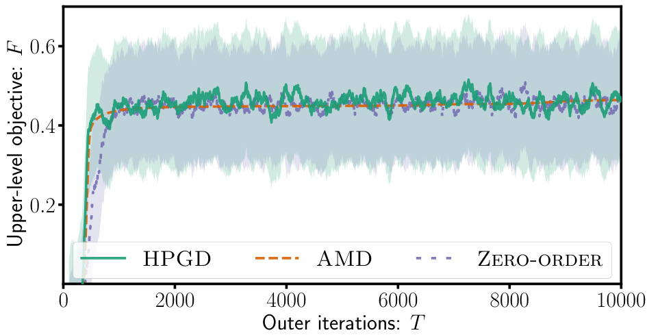
This figure shows the results of applying different algorithms (HPGD, AMD, Zero-Order) on a Four-Rooms environment. The left panel displays the state space of the environment, highlighting the start state (S), goal states (G1, G2), and target state (+1). The right panel shows the performance of each algorithm. HPGD outperforms AMD and Zero-Order, demonstrating its ability to navigate the state space effectively and avoid becoming stuck in local optima.
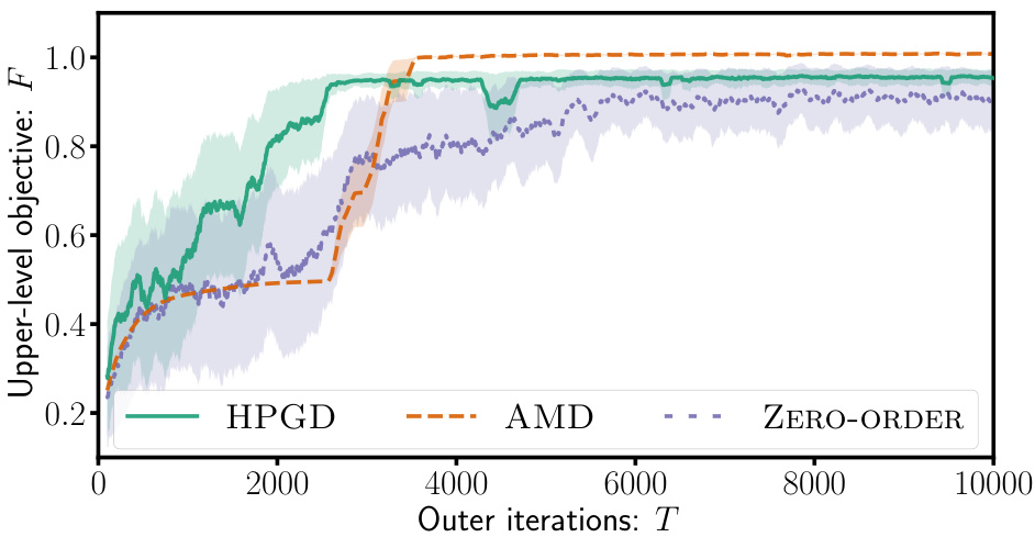
This figure consists of two subfigures. The left subfigure shows a grid-world environment called the Four-Rooms environment with a starting state (S), two goal states (G¹ and G²), and a target cell (+1). The right subfigure presents a performance comparison of three algorithms (HPGD, AMD, and Zero-Order) on the Four-Rooms environment, plotting the upper-level objective values over the number of outer iterations. It shows that HPGD surpasses AMD and Zero-Order, escaping local optima and achieving a better objective value.
The figure consists of two subfigures. The left subfigure shows the state space of the Four-Rooms environment, which is a grid world with four rooms and a goal in two different locations (G1 and G2). The agent starts in a designated start state (S) and the objective for the upper level is to guide the agent to a specific target state (+1). The right subfigure is a performance plot comparing HPGD against two other algorithms (AMD and Zero-Order) across outer iterations in terms of optimizing the upper-level objective function. This plot demonstrates that HPGD outperforms the other algorithms, especially by escaping local optima and achieving a higher value for the objective function.
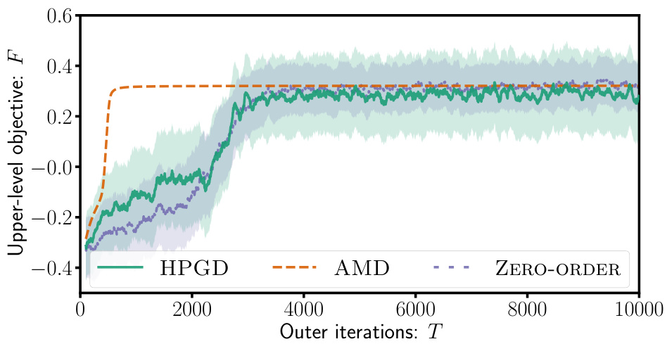
This figure shows the results of an experiment comparing the performance of three different algorithms (HPGD, AMD, and Zero-Order) on a Four-Rooms environment. The left panel displays the state space of the environment, showing the starting position (S), two goal states (G1 and G2), and the target cell (+1) that the upper-level algorithm aims to lead the lower-level agent to. The right panel presents a graph illustrating the performance of each algorithm over a certain number of iterations. It shows that HPGD is able to reach a higher objective value compared to the other algorithms, likely by escaping local optima.
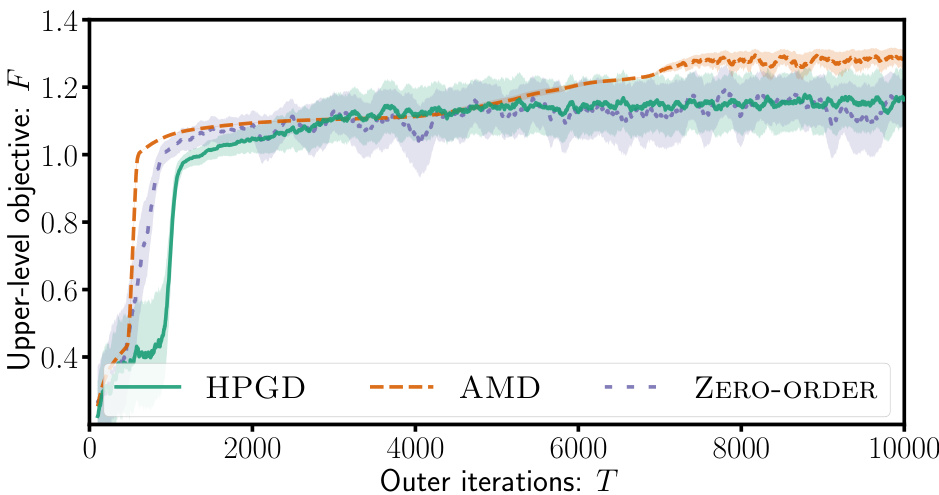
The figure contains two subfigures. The left subfigure shows the state space of the Four-Rooms environment. The right subfigure presents a comparison of the performance of three different algorithms (HPGD, AMD, and Zero-Order) in terms of the upper-level objective values over the number of outer iterations. The plot demonstrates that HPGD outperforms the other algorithms by escaping local optima and achieving a higher objective value.

This figure shows the results of the Four-Rooms experiment. The left panel shows a grid-world environment where the agent starts at S and must reach either goal state (G1 or G2). The +1 indicates the state the leader wants the follower agent to reach. The right panel displays the performance comparison of three algorithms in the Four-Rooms environment. HPGD outperforms the other two (AMD and Zero-Order) because of its ability to avoid getting stuck in local optima.
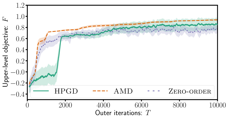
The figure shows two subfigures. The left subfigure displays the state space of the Four-Rooms environment used in the experiments. The right subfigure presents a performance comparison of three algorithms: HPGD, AMD, and Zero-Order. The algorithms aim to optimize the upper-level objective in the Four-Rooms environment by influencing the lower-level MDP. The plot shows the upper-level objective values over the number of outer iterations. HPGD outperforms the other two algorithms, escaping local optima and achieving better results.

This figure shows the reward penalties assigned to each state in the Four-Rooms environment by three different algorithms: HPGD, AMD, and Zero-Order. The penalties are represented by color intensity, with darker shades indicating stronger penalties. The algorithms aim to guide the lower-level agent towards a specific target state (+1) by strategically placing penalties. The figure visually compares the approaches of each algorithm in achieving this goal.

This figure shows the reward penalties assigned to states by three different algorithms (HPGD, AMD, and Zero-Order) in the Four-Rooms environment. The color intensity represents the magnitude of the penalty, with darker shades indicating stronger penalties. The goal is to guide the lower-level agent through a specific state (+1). The figure helps visualize how each algorithm modifies the environment to achieve its objective, highlighting differences in their approaches to reward shaping.

This figure shows the reward penalties assigned to each state in the Four-Rooms environment by three different algorithms: HPGD, AMD, and Zero-Order. The color intensity represents the magnitude of the penalty, with darker shades indicating stronger penalties. The figure visually compares how each algorithm uses penalties to influence the lower-level agent’s behavior, showcasing differences in their strategies for guiding the agent to a specific target location (+1).

This figure shows the reward penalties assigned by three different algorithms (HPGD, AMD, and Zero-Order) to influence the lower-level agent’s behavior in the Four-Rooms environment. The penalties, represented by color intensity, are designed to guide the agent towards a specific target cell (+1). The visualization helps to compare how each algorithm modifies the environment to achieve its objective, highlighting potential differences in their strategies and effectiveness.

This figure shows the reward penalties assigned by three different algorithms (HPGD, AMD, and Zero-Order) to the lower-level agent in each state of the Four-Rooms environment. The color intensity represents the magnitude of the penalty, with darker shades indicating stronger penalties. The algorithms aim to steer the lower-level agent through a specific target cell (+1). The figure illustrates how the different optimization strategies lead to varying penalty distributions across the states, reflecting the diverse ways in which the algorithms achieve their objective.

This figure visualizes the reward penalties assigned to each state by three different algorithms: HPGD, AMD, and Zero-Order. The goal is to guide the lower-level agent through a specific cell in the Four-Rooms environment. The color intensity represents the magnitude of the penalty, with darker shades indicating stronger penalties. The figure shows how each algorithm strategically applies penalties to influence the agent’s path.

This figure compares reward penalties assigned by three different algorithms (HPGD, AMD, and Zero-Order) in the Four-Rooms environment. Each algorithm aims to guide a lower-level agent toward a specific target cell (+1) by adjusting the reward penalties for each state. The color intensity represents the magnitude of the penalty. Darker shades indicate stronger negative penalties, while lighter shades show weaker penalties. The figure visualizes how each algorithm strategically uses penalties to influence the agent’s path, highlighting their differences in achieving the objective.

This figure compares the reward penalties assigned to different states in the Four-Rooms environment by three different algorithms: HPGD, AMD, and Zero-Order. The color intensity represents the magnitude of the penalty, with darker shades indicating stronger penalties. The goal is to observe how each algorithm shapes the reward function to guide the lower-level agent’s behavior. Specifically, the leader aims to influence the agent to pass through a particular cell (+1) en route to one of the goal states (G1 or G2). The figure helps to illustrate the differences in the approaches taken by each algorithm to solve this bilevel optimization problem.

This figure shows the results of applying the HPGD and Zero-Order algorithms to a tax design problem. The left panel displays the upper-level objective function (social welfare) over the number of outer iterations. HPGD converges to a higher social welfare value much faster than the Zero-Order method. The right panel displays the tax rates (income tax and VAT rates for three goods) over the outer iterations. HPGD efficiently learns to adjust tax rates to maximize social welfare, while the Zero-Order method takes significantly longer to find optimal rates and fails to distinguish between goods in setting optimal VAT rates.

This figure shows the performance of HPGD and Zero-Order algorithms on a tax design problem for macroeconomic models. The left panel displays the upper-level objective (social welfare) over the outer iterations, demonstrating that HPGD converges faster than Zero-Order. The right panel shows the evolution of tax rates (income tax and VAT rates for three goods) over iterations. HPGD efficiently adapts tax rates to maximize social welfare while Zero-Order struggles to learn optimal policies.
More on tables
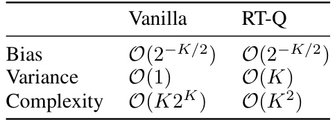
This table compares the key characteristics of several related works in bilevel reinforcement learning. It highlights differences in the use of context, side information, whether the leader’s control over the follower is agnostic or deterministic, the type of hypergradient updates (deterministic or stochastic), and the time complexity of the algorithm’s iterations at both the upper and lower levels. The table aids in understanding the novel contributions of the proposed HPGD algorithm in the paper by showing how it improves upon or differs from existing approaches.
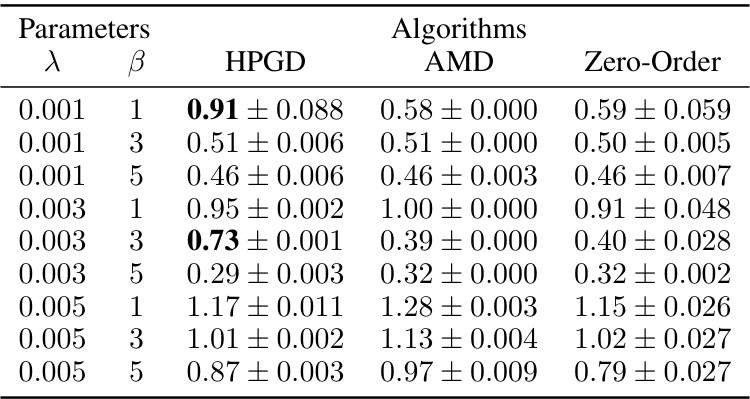
This table presents the performance of three different algorithms (HPGD, AMD, and Zero-Order) on the Four Rooms problem for various hyperparameter settings (λ and β). The results are averages over 10 random seeds, showing mean performance and standard errors. The table highlights that HPGD generally performs comparably to the other algorithms, but shows superior performance in a few instances, while also exhibiting more variance than AMD.
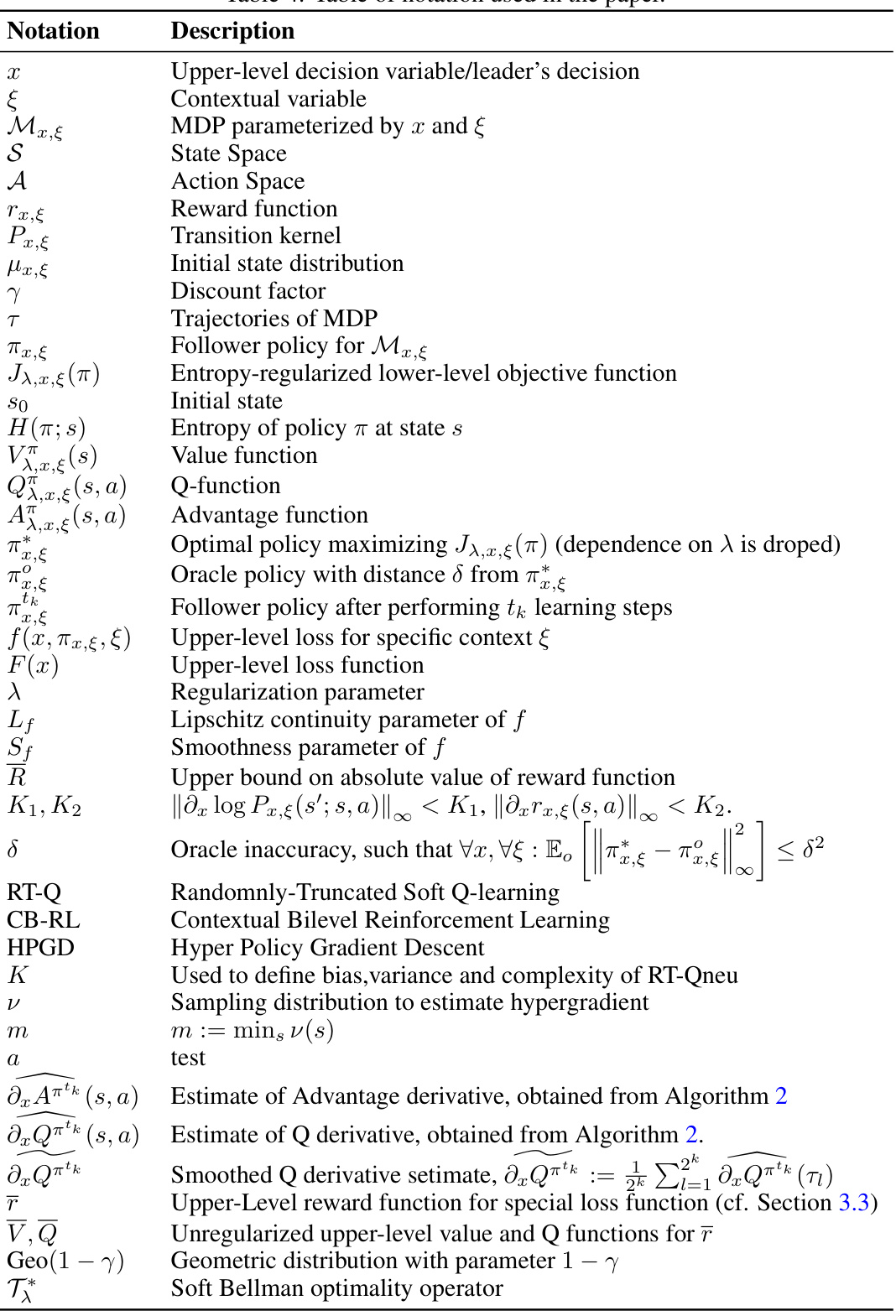
This table compares the key characteristics of several related works in bilevel reinforcement learning. It highlights the presence or absence of key features, such as contextual information, multiple followers, side information, whether the leader controls the followers’ training, whether algorithms are deterministic or stochastic, and the complexity of iterations for both upper and lower levels. This allows for a clear comparison of the proposed HPGD algorithm against existing approaches.

This table compares the key characteristics of several related works in bilevel reinforcement learning. It highlights the differences in the use of context, whether the leader’s algorithm is agnostic to the follower’s or not, the type of lower and upper level updates used (deterministic or stochastic), the number of iterations required at each level, and the specific algorithm employed. The table helps clarify the novel contributions of the proposed HPGD algorithm by showcasing its differences from existing methods.
Full paper#
