↗ OpenReview ↗ NeurIPS Homepage ↗ Chat
TL;DR#
Many real-world applications rely on Mixed-Integer Linear Programming (MILP), but improving MILP solvers requires vast amounts of high-quality data, which is often hard to obtain. Existing data generation methods often disrupt inherent problem structures, leading to computationally trivial or infeasible instances. This paper tackles this critical issue.
The researchers introduce MILP-StuDio, a novel framework that generates high-quality MILP instances by carefully preserving their block structures. This is achieved through block decomposition, a structure library, and three novel operators (removing, substituting, and appending block units). Experiments demonstrate MILP-StuDio’s ability to generate instances with flexible sizes while maintaining feasibility and computational hardness, thus significantly improving the performance of learning-based solvers.
Key Takeaways#
Why does it matter?#
This paper is crucial for researchers in operations research and machine learning due to its novel MILP instance generation framework, MILP-StuDio. It directly addresses the scarcity of high-quality MILP instances, a significant bottleneck for advancing MILP solvers. The framework’s ability to preserve crucial mathematical properties and scalability makes it highly impactful, opening doors for enhanced learning-based solver development and more robust benchmark creation. It is also relevant to researchers working with block-structured data which is very common in various application domains.
Visual Insights#

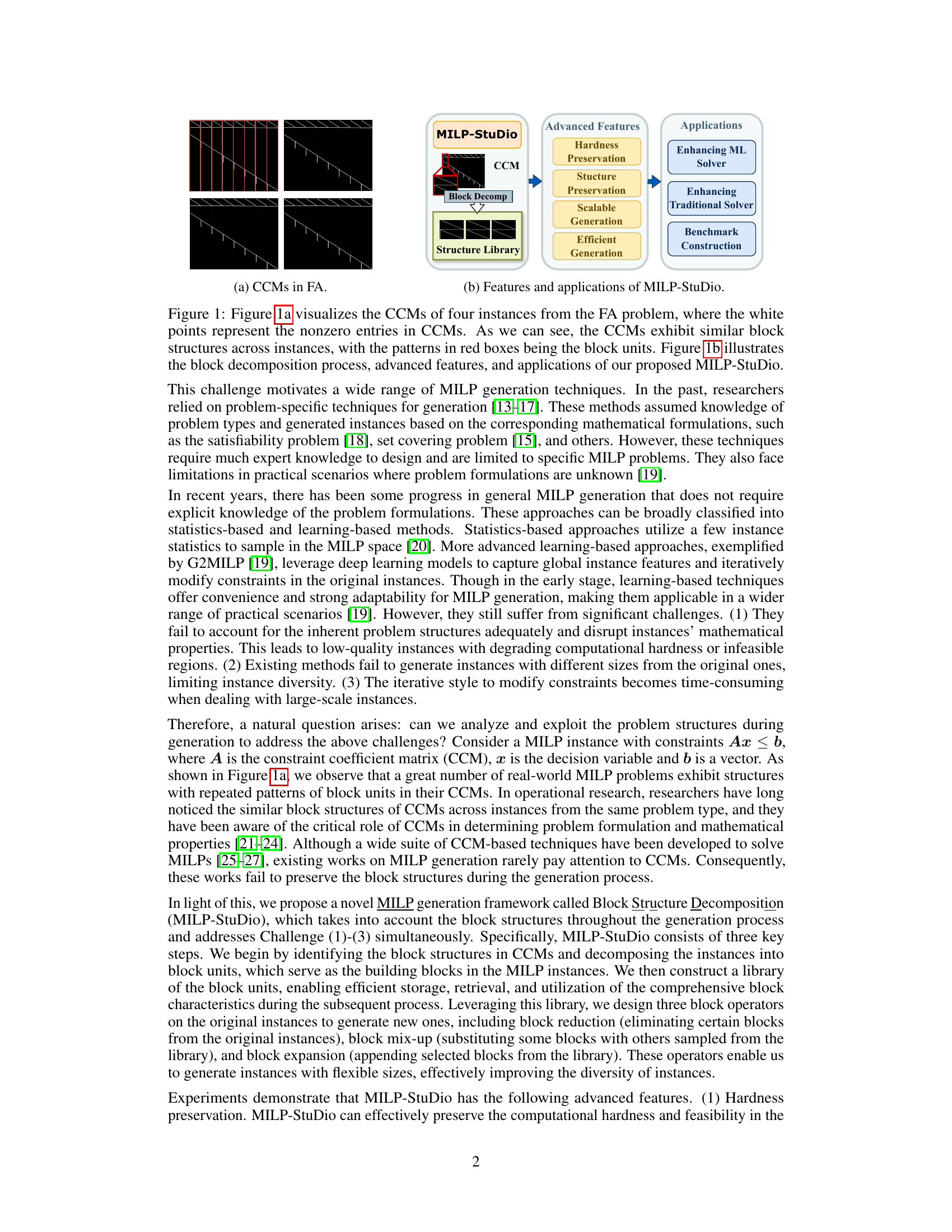
This figure visualizes the constraint coefficient matrices (CCMs) of MILP instances from four different benchmarks: Combinatorial Auctions (CA), Capacitated Facility Location (FA), Multiple Knapsacks (MIK), and Workload Appointment (WA). Each subfigure displays a visualization of the CCM for one benchmark, where the white points represent non-zero entries. The figure highlights the common presence of block structures within the CCMs across different instances of the same benchmark. This observation emphasizes that block structures are not unique to a single benchmark but are a widespread phenomenon in real-world MILP instances.

This table compares the performance of G2MILP, a learning-based MILP instance generation method, against the original instances. It shows the graph similarity (structural distributional similarity score), average solving time, and the proportion of feasible instances generated. The results highlight the challenges G2MILP faces in generating high-quality instances, particularly in maintaining feasibility.
In-depth insights#
MILP Block Structure#
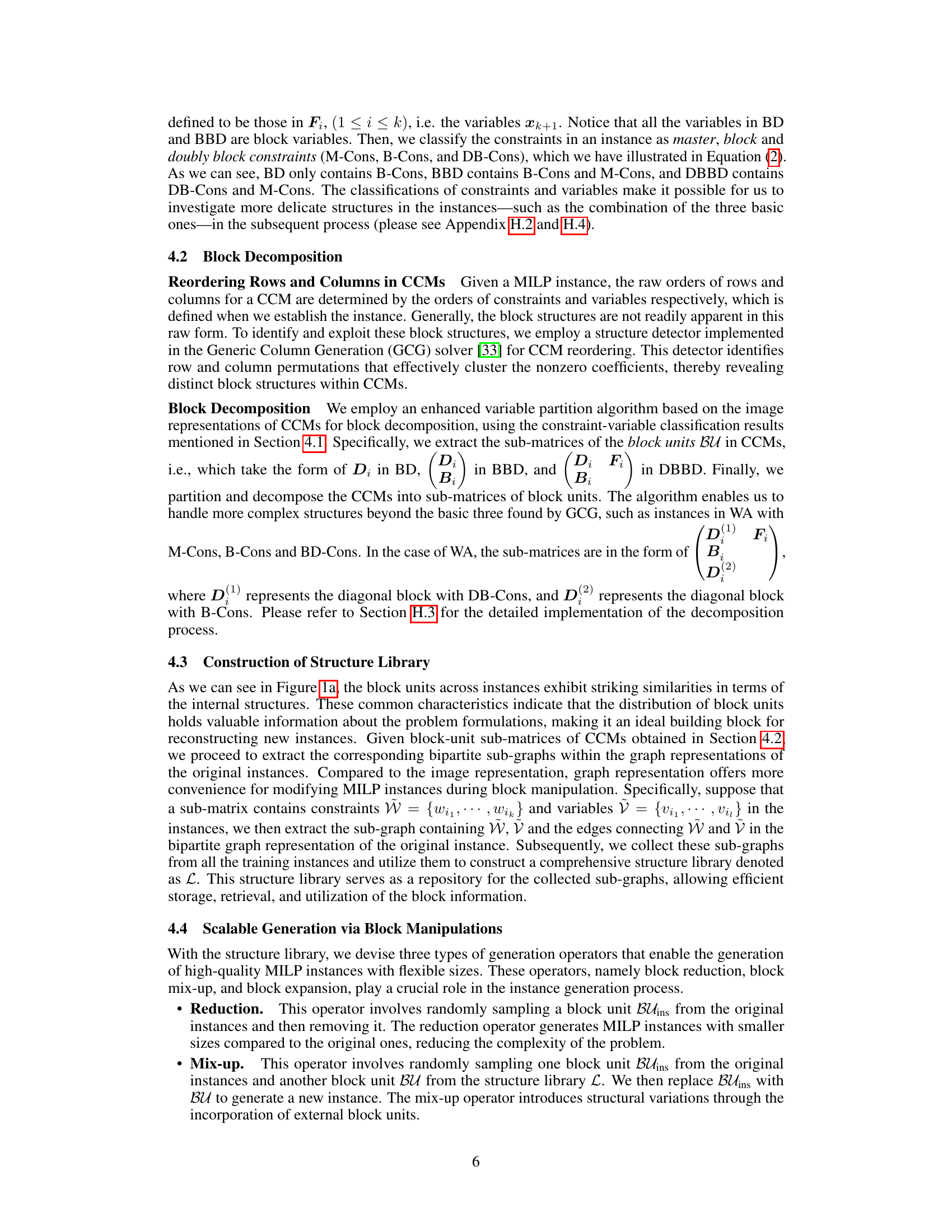
The concept of “MILP Block Structure” centers on the observation that in many real-world Mixed-Integer Linear Programming (MILP) problems, the constraint coefficient matrices (CCMs) exhibit recurring block patterns. These blocks represent substructures within the problem, often reflecting logical groupings of variables and constraints related to specific aspects of the modeled system. Understanding and leveraging these block structures is crucial because they often correlate with inherent mathematical properties of the MILP instance, impacting its computational hardness and solution characteristics. The presence of block structures provides opportunities for algorithmic improvements, such as the use of decomposition techniques (like Dantzig-Wolfe decomposition) that can significantly accelerate solution times. However, existing MILP instance generation techniques often fail to preserve or even recognize these critical structures. This oversight can lead to generated instances that lack realism or exhibit significantly different computational properties, hindering the development and evaluation of MILP solvers. Therefore, methods that explicitly consider and preserve block structures during instance generation are highly desirable. They are key to producing high-quality benchmarks that accurately reflect the complexities of real-world MILP problems and push forward the development of more effective algorithms.
StuDio Framework#
The hypothetical “StuDio Framework,” based on the provided context, likely centers on a novel approach to generating high-quality Mixed-Integer Linear Programming (MILP) instances. Its core innovation probably involves decomposing complex MILP instances into smaller, manageable “block units” which represent recurring patterns in the constraint coefficient matrices (CCMs). These units are stored in a library for efficient access, enabling flexible instance creation through operations like removing, substituting, or appending blocks. This method, therefore, addresses limitations in existing MILP instance generation techniques by preserving problem structure and ensuring feasibility, thus leading to more realistic and computationally challenging benchmark instances. The overall framework’s strength lies in its scalability and efficiency, creating various sized instances while maintaining computational hardness, ultimately improving the performance of both traditional and learning-based MILP solvers.
Block Manipulation#
The concept of ‘Block Manipulation’ in the context of MILP instance generation is crucial for creating high-quality and diverse instances. It involves techniques to modify or create new MILP instances by manipulating their underlying block structures, which are recurring patterns in the constraint coefficient matrices (CCMs). These manipulations are not random but carefully designed to preserve important mathematical properties such as feasibility and computational hardness, which are essential for evaluating MILP solvers. Different manipulation techniques can be used, such as removing, replacing, or adding blocks, leading to instances of varying sizes and complexity. The effectiveness of these manipulations depends on correctly identifying block units in the CCMs and using appropriate operators to modify them, hence the need for advanced feature preservation. The methods used must ensure that generated instances maintain a strong resemblance to real-world problems by retaining inherent structures and constraints, while simultaneously offering sufficient variability for effective solver training and evaluation. The key benefit lies in the controlled generation of realistic and challenging MILP instances tailored to specific needs, improving the training and benchmarking of MILP solvers.
Solver Enhancements#
Solver enhancements in the context of Mixed Integer Linear Programming (MILP) generally focus on improving the efficiency and effectiveness of algorithms used to solve these complex optimization problems. Key areas of enhancement often involve improved branching strategies, which determine the order in which variables are explored during the search process. Advanced cut generation techniques are another critical aspect; cuts are constraints that eliminate portions of the search space without removing any feasible solutions, thus accelerating convergence. Preprocessing steps can significantly reduce problem size and complexity before the main solution algorithm even begins. Beyond algorithmic improvements, learning-based approaches have shown promise, employing machine learning models to predict promising branching decisions, generate effective cuts, or even approximate solutions entirely, potentially achieving significant speedups over traditional methods. However, the success of learning-based techniques often hinges on the availability of high-quality training data, a challenge this paper addresses by presenting a novel MILP instance generation method.
Future Directions#
Future research could explore several promising avenues. Extending MILP-Studio’s applicability to a wider range of problem structures beyond those with readily identifiable block structures is crucial. This might involve developing more sophisticated block detection algorithms or exploring alternative representations of the constraint coefficient matrices. Another key area is improving the efficiency of the block decomposition and manipulation processes, potentially through parallelisation or more advanced heuristic methods. Investigating the impact of different types and sizes of block units on the quality of generated instances would provide valuable insights for optimising the instance generation strategy. Finally, exploring how MILP-Studio can be integrated into existing MILP workflows would enhance its practical value and allow researchers to easily incorporate high-quality, diverse instances into their work, potentially leading to significant improvements in learning-based and traditional solvers.
More visual insights#
More on figures

This figure shows two parts: (a) visualizes the constraint coefficient matrices (CCMs) of four instances from the capacitated facility location (FA) problem, highlighting the block structures; (b) illustrates the MILP-Studio framework, including its block decomposition process, advanced features (hardness and structure preservation, scalable and efficient generation), and applications (enhancing machine learning and traditional solvers, and benchmark construction).

This figure visualizes the constraint coefficient matrices (CCMs) of instances from four well-known MILP benchmarks: Combinatorial Auctions (CA), Capacitated Facility Location (FA), Multiple Knapsack (MIK), and Workload Appointment (WA). Each CCM is represented as a digital image where white pixels represent non-zero entries and black pixels represent zero entries. The images reveal that the CCMs across instances within each benchmark exhibit similar block structures, highlighting a key characteristic of real-world MILP problems that MILP-Studio leverages.

This figure visualizes the constraint coefficient matrices (CCMs) for instances from a MILP problem, illustrating the impact of different instance generation methods on the CCM structure. The left panel displays the CCM of an original instance, showing a clear block structure. The middle panel shows the CCM generated by G2MILP, exhibiting disrupted block structure and the introduction of noise. The right panel shows the CCM generated by MILP-StuDio, demonstrating its effectiveness in preserving the block structure.

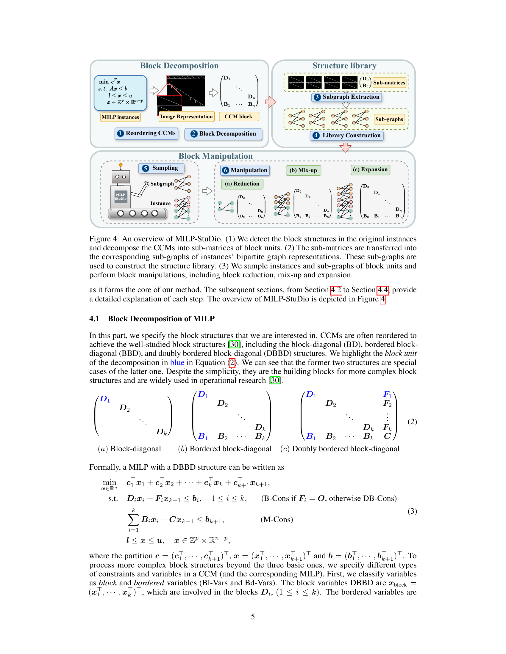
This figure illustrates the MILP-StuDio framework’s three main steps: block decomposition, structure library construction, and block manipulation. First, block structures within the constraint coefficient matrices (CCMs) of the input MILP instances are identified and decomposed into sub-matrices representing block units. These sub-matrices are then converted into sub-graphs based on the instances’ bipartite graph representations. These sub-graphs are stored in a structure library. Finally, block manipulation operators (reduction, mix-up, and expansion) are applied to the original instances by sampling from the structure library to generate new MILP instances with varying sizes and complexities, while maintaining structural properties.

This figure illustrates the MILP-StuDio framework’s three main steps: block decomposition, structure library construction, and block manipulation. It shows how the algorithm identifies block structures in constraint coefficient matrices (CCMs), converts them to sub-graphs for a library, and uses three operators (reduction, mix-up, and expansion) to create new MILP instances by modifying these blocks.
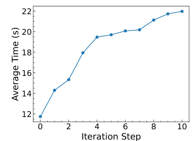
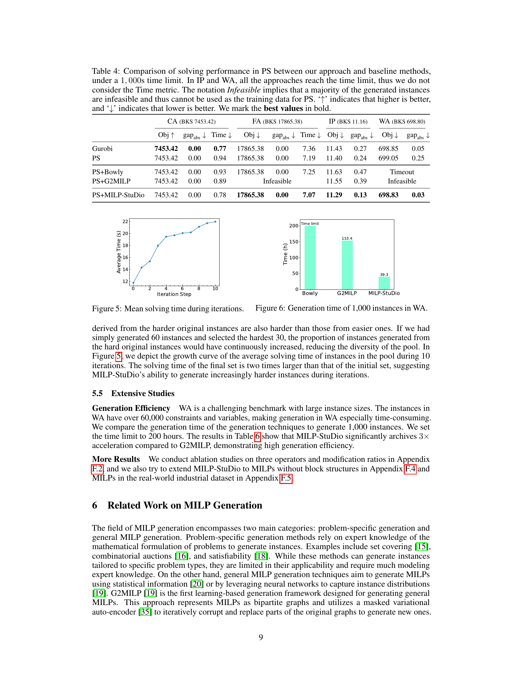
The figure shows a line graph depicting the average solving time over 10 iterations. The average solving time gradually increases with each iteration, indicating that the generated instances become progressively harder to solve. This demonstrates MILP-StuDio’s ability to generate increasingly challenging instances.

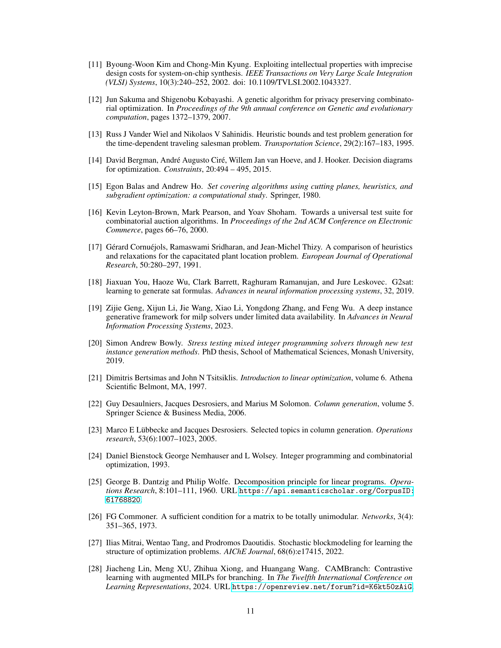
This figure shows the time it takes to generate 1000 instances of the Workload Appointment (WA) problem using three different methods: Bowly, G2MILP, and MILP-Studio. MILP-Studio is significantly faster than the other two methods, highlighting its efficiency in generating large-scale MILP instances.

This figure visualizes the constraint coefficient matrices (CCMs) of four different sets of instances from the Combinatorial Auctions (CA) problem. The top left image shows the CCM of an original instance. The other three images display the CCMs generated by different methods: Bowly, G2MILP, and the proposed MILP-StuDio. The goal is to illustrate how each method affects the structure of the CCM, and whether it preserves the structural properties or introduces noise or distortions.
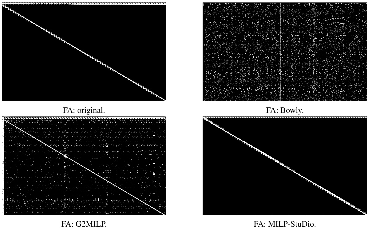
The figure visualizes the constraint coefficient matrices (CCMs) of four instances from the capacitated facility location (FA) problem. The top-left image shows a CCM from an original FA instance, exhibiting a clear block structure. The subsequent images visualize CCMs generated by three different methods: Bowly, G2MILP, and the proposed MILP-StuDio. The goal is to show how well each method preserves or distorts the block structure of the original instances. Visual inspection reveals that MILP-StuDio most closely maintains the block structure of the original CCM, while Bowly and G2MILP introduce significant changes or noise, respectively.

The figure visualizes the constraint coefficient matrices (CCMs) of the original and generated instances from the item placement (IP) problem benchmark. The visualization helps compare the structure of the CCMs. It shows how well each instance generation method preserves the original structure and the degree of noise or disruption introduced by each method. This is important for understanding the quality of generated instances for training machine learning-based solvers. The CCMs are represented as images, where white points represent non-zero entries. The top left image shows the original IP instance’s CCM. The images on the right show the CCMs of instances generated using the Bowly, G2MILP, and MILP-Studio methods.

This figure visualizes the constraint coefficient matrices (CCMs) of MILP instances from the WA benchmark. It compares the CCMs of original instances to those generated using three different methods: Bowly, G2MILP, and MILP-StuDio. The Bowly method failed to complete due to excessive computation time. The visualizations highlight how MILP-StuDio effectively preserves the block structures present in the original instances, unlike G2MILP, which introduces noise that disrupts these structures. This illustrates MILP-StuDio’s ability to generate high-quality instances by preserving important structural characteristics.

This figure provides a visual overview of the MILP-Studio framework. It shows the three main stages: Block Decomposition (identifying and separating block structures in the constraint coefficient matrix), Structure Library (creating a library of reusable block units), and Block Manipulation (using operators to create new instances by combining, removing, or adding block units from the library).
More on tables

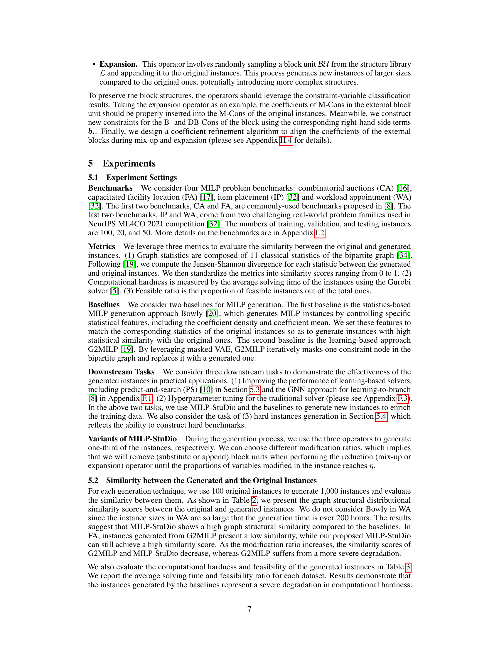
This table presents the structural distributional similarity scores achieved by different MILP instance generation methods (Bowly, G2MILP, and MILP-Studio) across four benchmark datasets (CA, FA, IP, WA). Higher scores indicate greater similarity between the generated and original instances. The ‘Timeout’ entry indicates that the generation process exceeded the 200-hour time limit.

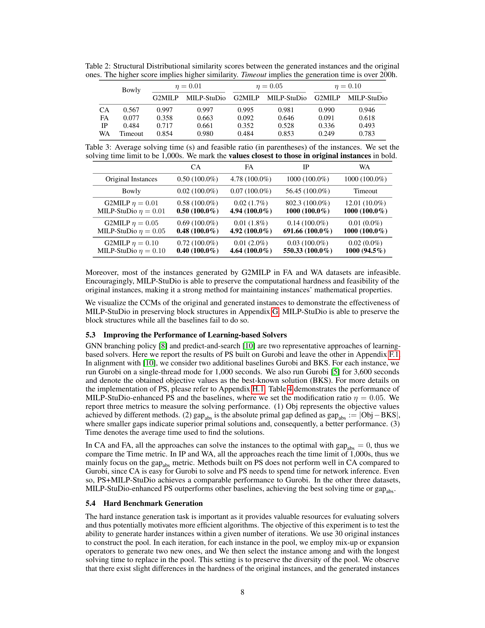
This table compares the average solving time and the percentage of feasible instances generated by different methods (Bowly, G2MILP, and MILP-Studio with different modification ratios) against the original instances across four benchmark datasets (CA, FA, IP, and WA). The solving time limit was set to 1000 seconds. The table highlights that MILP-Studio consistently maintains a higher feasible ratio and closer solving times to the original data, indicating the method’s success in preserving the properties of the original instances.

This table compares the performance of different MILP instance generation methods on four benchmark datasets (CA, FA, IP, WA). The metrics used are the average solving time (with a 1000-second time limit) and the percentage of feasible instances generated. The goal is to assess which method best preserves the computational hardness and feasibility of the original instances.
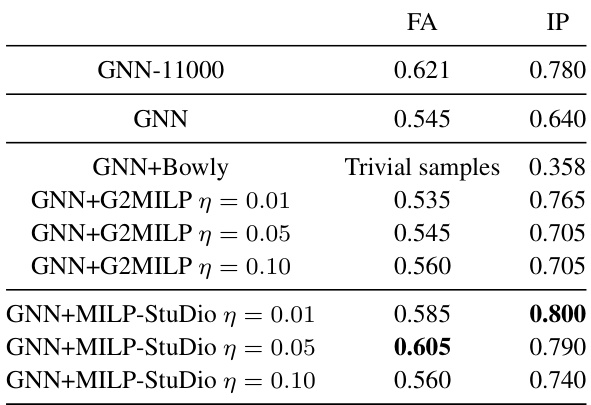
This table presents the branching accuracy results on testing datasets for several methods. The methods involve training a Graph Neural Network (GNN) for branching decisions using different data generation techniques (GNN-11000, GNN, GNN+Bowly, GNN+G2MILP, GNN+MILP-StuDio). The table shows that MILP-StuDio consistently leads to better branching accuracy compared to the other data generation methods. Note that some methods resulted in trivial samples, meaning the generated instances were too simple to require branching.
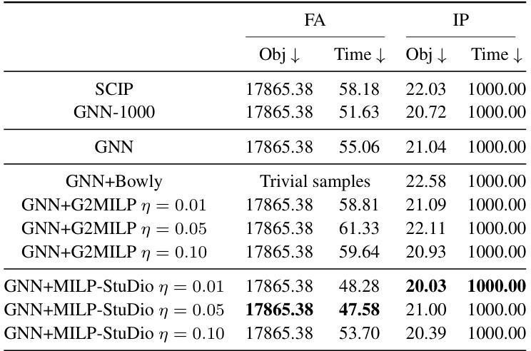
This table compares the performance of learning-to-branch models trained on instances generated by different methods (GNN, GNN+Bowly, GNN+G2MILP, GNN+MILP-Studio) and the original instances. The performance is measured by the objective values (Obj) and solving times (Time). Lower values for both Obj and Time are better. The table shows that MILP-Studio consistently improves the performance of the learning-to-branch model.

This table shows the structural similarity scores between instances generated by different methods (G2MILP and MILP-Studio with different operators and modification ratios) and the original instances for the FA dataset. The mix-up operator in MILP-Studio consistently achieves the highest similarity scores, suggesting it produces instances most similar to the real-world data.

This table shows the average time taken by the Gurobi solver to solve instances generated using different methods and modification ratios. It also shows the percentage of generated instances that were feasible (i.e., had a valid solution). The results highlight that G2MILP struggles to generate feasible instances, unlike the proposed MILP-Studio method.

This table compares the prediction loss on testing datasets for the Predict and Search algorithm using instances generated by different operators in the MILP-Studio framework. The modification ratio (η) is set to 0.05 for all methods. The best performance for each benchmark (FA and IP) is highlighted in bold. This helps to evaluate the impact of the different generation operators on the performance of the Predict and Search algorithm.
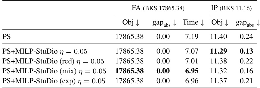
This table compares the performance of the Predict-and-Search (PS) algorithm when using different block manipulation operators within the MILP-Studio framework. It shows the objective value, absolute gap from the best-known solution, and solving time for the FA (capacitated facility location) and IP (item placement) benchmark problems. The results indicate the effectiveness of different operators in improving the PS algorithm’s performance.

This table presents the prediction loss results for the Predict-and-Search (PS) algorithm using instances generated with different modification ratios (0.01, 0.05, and 0.10) by both G2MILP and MILP-Studio. The results are broken down by dataset (FA and IP). The ‘infeasible’ label indicates that the generated instances were mostly infeasible and therefore unusable for training. The table highlights the superior performance of MILP-Studio across all modification ratios and datasets, demonstrating its ability to generate high-quality, feasible instances.

This table compares the performance of different methods in solving the learning-to-branch task using the FA and IP benchmarks. The methods include the original GNN model trained on a subset of instances and GNN models trained on instances generated by different methods (Bowly, G2MILP, and MILP-Studio) with various modification ratios. The table shows the objective values and average solving times for each method and dataset. The ‘Trivial samples’ entry notes instances where the computational hardness was too low to require branching.

This table presents the graph structural distributional similarity scores between generated and original instances for four different MILP datasets (CA, FA, IP, WA) using three different generation methods (Bowly, G2MILP, MILP-Studio) and three different modification ratios (0.01, 0.05, 0.10). A higher score indicates greater similarity between the generated and original instances’ structures. The ‘Timeout’ indicates that the generation time exceeded 200 hours for the Bowly method on the WA dataset.
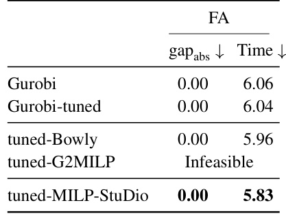
This table presents the results of hyperparameter tuning for the Gurobi solver using different instance generation methods. The ‘gapabs’ column shows the absolute difference between the objective function value found by Gurobi and the best-known solution (BKS). The ‘Time’ column shows the average solving time in seconds. The results demonstrate that tuning Gurobi with instances generated by MILP-StuDio leads to a significant improvement in solving time, achieving the best performance among all methods tested.

This table compares the similarity, solving time, and feasibility of instances generated by different methods against the original instances from the Setcover benchmark. The metrics assess how well each method preserves the characteristics of the original instances. The solving time is capped at 300 seconds, and the modification ratio (η) is set to 0.05. MILP-Studio demonstrates superior performance in maintaining the characteristics of the original data.

This table compares the performance of the Predict-and-Search (PS) algorithm using instances generated by different operators of the MILP-StuDio framework. It shows the objective value achieved (Obj), the absolute gap between that objective and the best-known solution (gapabs), and the time taken to find the solution (Time). The results indicate that the MILP-StuDio framework improves the performance of PS, regardless of the specific operator used.

This table presents a comparison of the similarity scores, solving times, and feasibility ratios for the original MIS instances and those generated using three different methods: Bowly, G2MILP, and MILP-StuDio. The solving time limit was set to 300 seconds, and the modification ratio (η) was 0.05. The best performing method for each metric is highlighted in bold. The results show that MILP-StuDio and G2MILP generate instances with high similarity to the originals, while maintaining 100% feasibility, unlike Bowly which had significantly faster solving times.

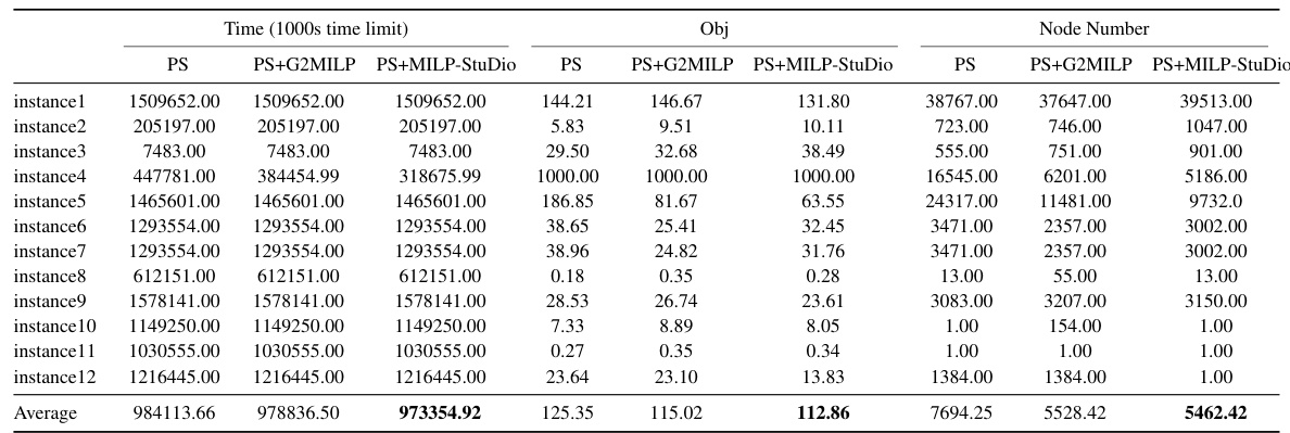
This table compares the performance of the Predict-and-Search (PS) solver when trained using instances generated by different methods (Gurobi, PS, Bowly, G2MILP, and MILP-Studio). The performance is evaluated on a non-structural MIS benchmark with a 300-second time limit and a modification ratio of 0.05. The metrics reported include solving time, objective value, and the absolute gap between the objective value and the best-known solution.
This table compares the average solving time and the percentage of feasible instances generated by different methods (Bowly, G2MILP, and MILP-StuDio with different modification ratios) against the original instances. The solving time is capped at 1000 seconds. The bold values indicate which generated instances are closest to the original data in terms of solving time. This provides a measure of how well each method preserves the computational hardness of the original MILP instances.

This table shows the values of hyperparameters used in the Predict-and-Search (PS) algorithm for different benchmarks (CA, FA, IP, WA). These hyperparameters control the size of the partial solution considered and the search neighborhood explored during the solving process.

This table presents the structural distributional similarity scores between the generated instances and the original instances for four different MILP problem benchmarks (CA, FA, IP, WA). The similarity scores are calculated using 11 graph statistics to measure the similarity between the original and generated instances and are shown for three different modification ratios (η = 0.01, η = 0.05, η = 0.10). Higher scores indicate greater similarity. For the WA benchmark, the generation time exceeded 200 hours for one method.

This table presents the structural distributional similarity scores between the generated instances and the original instances for four different MILP datasets (CA, FA, IP, WA). The similarity is calculated using 11 graph statistics. A higher score indicates greater similarity between the generated and original instances. The table also notes when the generation time exceeded 200 hours, indicating that the generation process did not complete for those instances.

This table presents a statistical summary of four MILP problem benchmarks used in the paper: Combinatorial Auctions (CA), Capacitated Facility Location (FA), Item Placement (IP), and Workload Appointment (WA). For each benchmark, the table provides the number of constraints, the number of variables, the number of blocks identified in the constraint coefficient matrices (CCMs), the types of constraints (M-Cons, B-Cons, D-Cons, DB-Cons), and the types of variables (Bl-Vars, Bd-Vars). This information is crucial for understanding the characteristics of the datasets and for comparing the performance of different MILP generation methods.

This table presents the structural distributional similarity scores between instances generated by different methods and the original instances. The similarity is measured using 11 graph statistics, and a higher score indicates greater similarity. The table shows results for four different datasets (CA, FA, IP, WA) and three different modification ratios (η = 0.01, 0.05, 0.10) for each method. The ‘Bowly’, ‘G2MILP’, and ‘MILP-StuDio’ methods are compared. Note that for the WA dataset, the Bowly method timed out, meaning it took over 200 hours to complete.
Full paper#
