↗ OpenReview ↗ NeurIPS Homepage ↗ Chat
TL;DR#
Deep Operator Networks (DeepONets) are effective surrogate models for parametric partial differential equations (PDEs). However, they often struggle to accurately approximate solution derivatives, especially when training data is scarce. This paper introduces Derivative-enhanced DeepONets (DE-DeepONets) to address this limitation. The key issue is that existing neural operators do not provide accurate estimates of the derivative of the output with respect to the input, which is necessary for many downstream tasks.
DE-DeepONets improve upon DeepONets by incorporating derivative information into the training process and using a dimension reduction technique to reduce computational cost and improve training efficiency. Numerical experiments demonstrate that DE-DeepONets outperform existing methods in terms of both accuracy and computational efficiency, particularly when the amount of training data is limited. Furthermore, the approach can easily be generalized to other neural operators such as the Fourier Neural Operator (FNO).
Key Takeaways#
Why does it matter?#
This paper is important because it significantly improves the accuracy of Deep Operator Networks (DeepONets), a popular method for solving many-query problems involving partial differential equations (PDEs). The enhanced accuracy, particularly beneficial with limited data, opens new avenues in various applications, including Bayesian inference, optimization under uncertainty, and experimental design. This work is especially relevant to the growing field of physics-informed machine learning. The new method, DE-DeepONet, is also shown to be easily adapted to other neural operators, thus greatly increasing the usefulness and applicability of this approach.
Visual Insights#
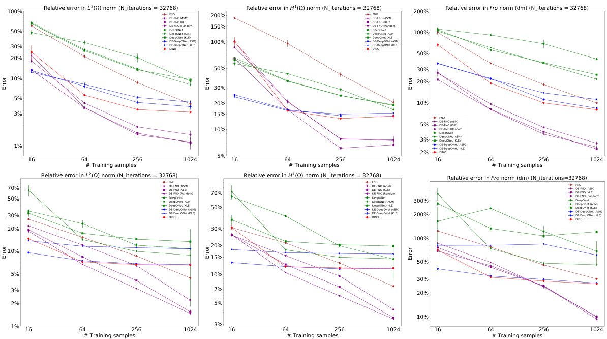
This figure compares the performance of different neural operator methods (DeepONet, FNO, DINO, and DE-DeepONet) on two different PDEs, hyperelasticity and Navier-Stokes, with varying numbers of training samples. The plots show the relative error in L2 and H1 norms for solution prediction and the relative error in the Frobenius norm for the prediction of the solution’s derivative with respect to the input parameter. The results highlight the improved accuracy of the DE-DeepONet, especially with limited training data.

This table shows the relative L2 error for output reconstruction using KLE and ASM basis with 16 input reduced bases for both hyperelasticity and Navier-Stokes datasets. It demonstrates the impact of the chosen dimension reduction technique on the accuracy of the output approximation. The lower error values indicate a better approximation using the selected dimension reduction method.
In-depth insights#
Derivative DeepONets#
Derivative DeepONets represent a significant advancement in the field of neural operators by leveraging derivative information to enhance accuracy and efficiency. The core idea is to incorporate derivative information explicitly into the DeepONet architecture, moving beyond simply approximating the solution to also accurately approximating its derivative with respect to input parameters. This is particularly beneficial when training data is scarce, a common challenge in many scientific applications of DeepONets. The enhanced accuracy comes from a better representation of the solution manifold, allowing for more accurate predictions, especially concerning derivatives crucial for downstream tasks like optimization or uncertainty quantification. By incorporating derivative loss into the training process, the model is further guided towards approximating both the solution and its derivative effectively, resulting in improved performance with potentially fewer training samples. While computationally more expensive in training due to derivative calculations, the resulting enhanced accuracy and efficient evaluation, particularly regarding derivatives, makes Derivative DeepONets a powerful tool in a variety of applications, especially when the cost of acquiring high-fidelity solutions and derivatives is substantial.
Dimension Reduction#
The concept of dimension reduction is crucial for handling high-dimensional data, a common challenge in many-query problems involving parametric PDEs. The paper explores this challenge, particularly in the context of enhancing DeepONet’s performance. Two primary dimension reduction techniques are investigated: Karhunen-Loève Expansion (KLE) and Active Subspace Method (ASM). KLE, an established method, provides an optimal basis for minimizing mean-square error, while ASM focuses on identifying input directions with the most significant impact on output variability. The paper highlights the computational advantages of ASM, showcasing its ability to reduce the dimension of the parameter input vector ’m’ (from Nin to r, with r < Nin), thereby minimizing the computational burden of the loss function. This reduction significantly improves efficiency without compromising prediction accuracy, especially when training data is limited. The choice between KLE and ASM is presented as a trade-off, with KLE offering simplicity but potentially lower accuracy in comparison to the more computationally intensive ASM which captures essential input-output sensitivity.
Active Subspace#
Active subspace methods are powerful dimension reduction techniques particularly useful when dealing with high-dimensional parameter spaces in partial differential equations (PDEs). They identify the most influential directions in the parameter space that significantly impact the output variance, effectively reducing computational complexity and improving model efficiency. The method leverages the gradient information of the output with respect to the input parameters, constructing a sensitivity matrix. Eigen-decomposition of this matrix reveals the active subspace, a low-dimensional subspace that captures most of the output variability. By projecting the high-dimensional input into this active subspace, one drastically reduces the dimensionality of the problem while retaining crucial information for accurate model predictions. The efficiency gains are particularly significant when solving computationally expensive PDEs repeatedly for various parameters, as often encountered in uncertainty quantification, optimization, and Bayesian inference problems. The primary advantage is the ability to substantially lower the computational cost without sacrificing too much accuracy. While computationally more intensive than other methods like Karhunen-Loève expansion (KLE), ASM’s ability to capture sensitivity provides superior performance in high-dimensional, nonlinear scenarios. However, the computational cost of ASM remains relatively high, especially for complex models and large datasets, presenting a limitation to its applicability in some real-world situations.
Derivative Loss#
The concept of ‘Derivative Loss’ in the context of neural operators for solving partial differential equations (PDEs) is a crucial innovation. It addresses the limitation of standard neural operator architectures, which often struggle to accurately predict not only the solution but also its derivatives with respect to parameters. By explicitly incorporating a derivative loss term into the overall loss function, the training process is guided to learn a more accurate representation of the solution’s sensitivity. This is particularly valuable when training data is scarce because accurate derivative information can significantly boost the model’s performance and generalization capabilities. The inclusion of derivative loss enhances the quality of the solution itself, as the model is forced to capture the underlying functional relationships more precisely. It also proves beneficial for various downstream tasks requiring sensitivity information, such as Bayesian inference or PDE-constrained optimization. However, implementing derivative loss presents challenges, especially with the high dimensionality often associated with PDEs. This is addressed by utilizing dimension reduction techniques, which reduces computational complexity and addresses the problem of storing and manipulating large Jacobian matrices. The effectiveness of derivative loss is further demonstrated through numerical experiments, showcasing its advantage over traditional methods in several case studies. In conclusion, derivative loss is a powerful technique that improves the accuracy and applicability of neural operators solving PDEs, particularly where data is limited.
PDE Enhancements#
The heading ‘PDE Enhancements’ suggests improvements made to the solution or approximation of Partial Differential Equations (PDEs). A thoughtful analysis would explore how these enhancements are achieved, focusing on their novelty and impact. This might involve novel numerical methods, machine learning techniques, or a combination of both. For example, enhancements could focus on improving accuracy, efficiency (faster computation times), or handling of complex scenarios such as high dimensionality or uncertainty. Specific examples might include using derivative information to improve model training data or employing dimension reduction methods to speed up calculations. The effectiveness and limitations of the approach must also be critically evaluated, comparing it to existing methods. Key insights would lie in understanding what types of PDE problems benefit most from these enhancements and the underlying reasons for their success. Finally, future research directions suggested by the enhancements would be a valuable contribution. Overall, a thorough discussion of ‘PDE Enhancements’ necessitates a detailed explanation of the methods, their advantages, limitations, and implications for the broader field of PDE research.
More visual insights#
More on figures

This figure compares the performance of different neural operator methods (DeepONet, FNO, DINO, and DE-DeepONet) in approximating the solution and its derivative with respect to the input parameter for two PDEs: hyperelasticity (top row) and Navier-Stokes (bottom row). The left column shows the relative L² error, the middle column shows the relative H¹ error, and the right column shows the relative Frobenius norm error of the derivative. The x-axis represents the number of training samples used, and the y-axis represents the relative error. The plots show how the accuracy of each method improves as more training data becomes available. DE-DeepONet consistently shows superior performance.
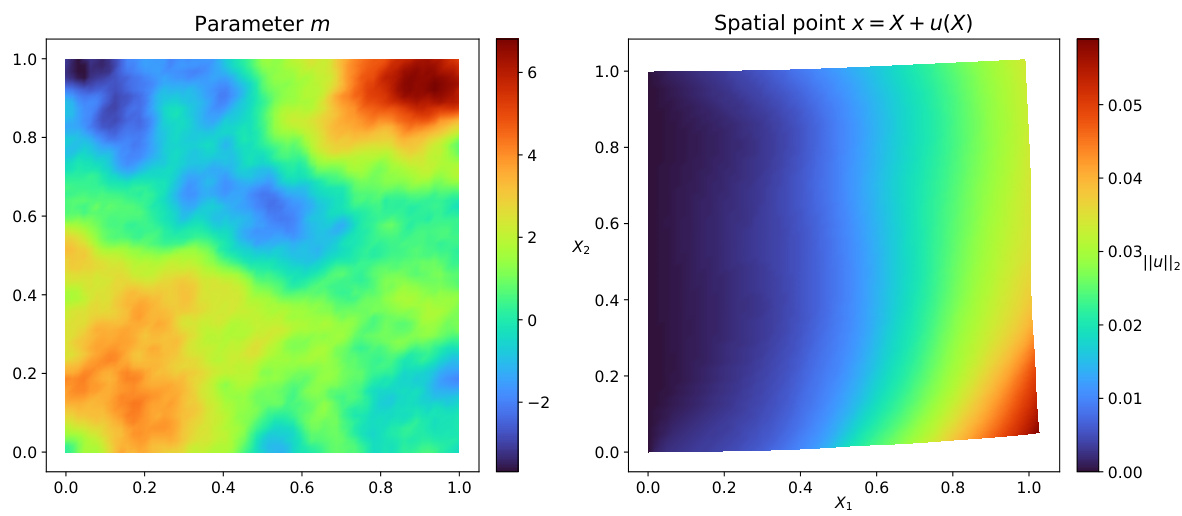
This figure visualizes a single sample from the hyperelasticity equation’s solution space. The left panel shows the input parameter m as a 2D heatmap. The right panel displays the resulting spatial point x after deformation, calculated as x = X + u(X), where X is the original material point and u is the displacement. The color scale represents the L2 norm of the displacement vector. Additional figures (13 and 14) in the paper provide visualizations of the displacement components u1 and u2 separately.

This figure visualizes a single parameter-solution pair from the Navier-Stokes equations. It shows three 2D plots: the first plot displays the random field representing the parameter (viscosity term), the second shows the x-component of the velocity field, and the third shows the y-component of the velocity field. The color scales are used to represent the magnitude of each quantity across the domain. This visualization provides a snapshot of the solution’s behavior for a specific parameter value.
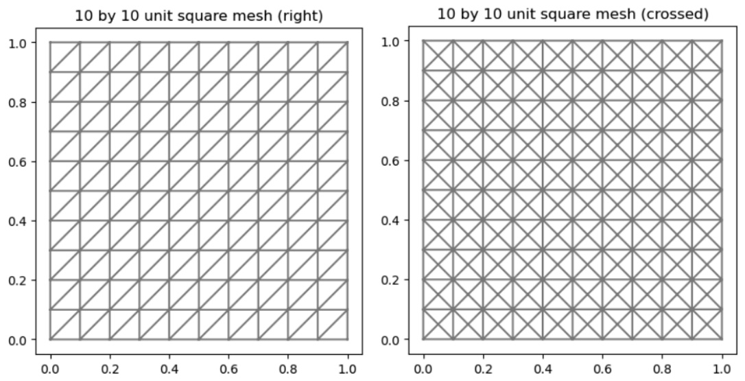
This figure shows two different triangular meshes of a 2D unit square with a resolution of 10 by 10. The left panel shows a mesh where the diagonals of the squares are oriented from bottom-left to top-right (‘right’), while the right panel shows a mesh where the diagonals are oriented from bottom-left to top-right and top-left to bottom-right (‘crossed’). These are common types of meshes used in the finite element method to approximate solutions of partial differential equations.

This figure compares the performance of different methods (DeepONet, FNO, DINO, DE-DeepONet) for solving two nonlinear PDEs (hyperelasticity and Navier-Stokes) with varying numbers of training samples. The plots show the relative errors in L2 and H1 norms for the solution prediction and Frobenius norm for the derivative prediction. It demonstrates the impact of training sample size on the accuracy of different methods, highlighting the superior performance of DE-DeepONet when training samples are limited.

This figure compares the performance of different neural operator methods (DeepONet, FNO, DINO, DE-DeepONet) for solving two nonlinear PDEs: hyperelasticity and Navier-Stokes. It shows the relative errors in L², H¹, and Frobenius norms for the prediction of the solution (u) and its derivative (∇mu) with respect to the input parameter. The x-axis represents the number of training samples, demonstrating how the accuracy improves with more data. The results reveal that DE-DeepONet consistently outperforms other methods, especially when training data is limited.

This figure compares the performance of different neural operator methods (DeepONet, FNO, DINO, and DE-DeepONet) for solving two nonlinear PDEs: hyperelasticity and Navier-Stokes. It shows the relative errors in L2 and H1 norms for the solution prediction and the relative error in the Frobenius norm for the derivative prediction. The results are presented for different numbers of training samples, illustrating the impact of data size on accuracy.

This figure compares the performance of different methods (DeepONet, FNO, DINO, DE-DeepONet) for solving two PDEs (hyperelasticity and Navier-Stokes) with varying amounts of training data. The plots show the relative error in the L2 and H1 norms for the solution prediction, and the relative Frobenius norm error for the prediction of the solution’s derivative with respect to the input parameters. The results indicate the impact of training sample size on the accuracy of different methods.

This figure compares the performance of different methods (DeepONet, FNO, DINO, DE-DeepONet) for solving the hyperelasticity and Navier-Stokes equations. It shows how the relative errors in L2 and H1 norms for the solution (u) and the Frobenius norm for the Jacobian (∇mu) change with the number of training samples. The top row displays results for the hyperelasticity equation, while the bottom row shows results for the Navier-Stokes equation. Each column represents a different error metric.

This figure compares the performance of different neural operator methods (DeepONet, FNO, DINO, DE-DeepONet) for solving two nonlinear PDEs: hyperelasticity and Navier-Stokes. It shows the relative error in L², H¹, and Frobenius norms for different numbers of training samples. The results demonstrate the improved accuracy of DE-DeepONet, especially when training data is limited.

This figure compares the performance of different neural operator methods (DeepONet, FNO, DINO, and DE-DeepONet) in approximating solutions of the hyperelasticity and Navier-Stokes equations. It shows the relative errors in L² and H¹ norms for the solution and Frobenius norm for the derivative, plotted against the number of training samples. The results indicate the effectiveness of DE-DeepONet, particularly when training data is limited.

This figure compares the performance of different neural operator methods (DeepONet, FNO, DINO, and DE-DeepONet) on two nonlinear PDEs: hyperelasticity and Navier-Stokes. It shows the relative errors in L2 and H1 norms for the solution prediction and the relative error in the Frobenius norm for the derivative prediction, as a function of the number of training samples. The results are averaged over 5 random seeds and show standard deviations.

This figure compares the performance of different neural operator methods (DeepONet, FNO, DINO, and DE-DeepONet) for solving two nonlinear PDEs: hyperelasticity and Navier-Stokes. It shows the relative error in L² and H¹ norms for the solution prediction, as well as the Frobenius norm error for the derivative prediction with respect to the input parameters. The x-axis represents the number of training samples, while the y-axis represents the relative error. The results are averaged over 5 independent runs.
This figure compares the performance of different neural operator methods (DeepONet, FNO, DINO, DE-DeepONet) for solving two nonlinear PDEs (hyperelasticity and Navier-Stokes equations). It shows the relative errors in L2 and H1 norms for the solution prediction and the Frobenius norm for the derivative prediction against the number of training samples. The results indicate that DE-DeepONet generally achieves the best accuracy, especially when training data is limited.
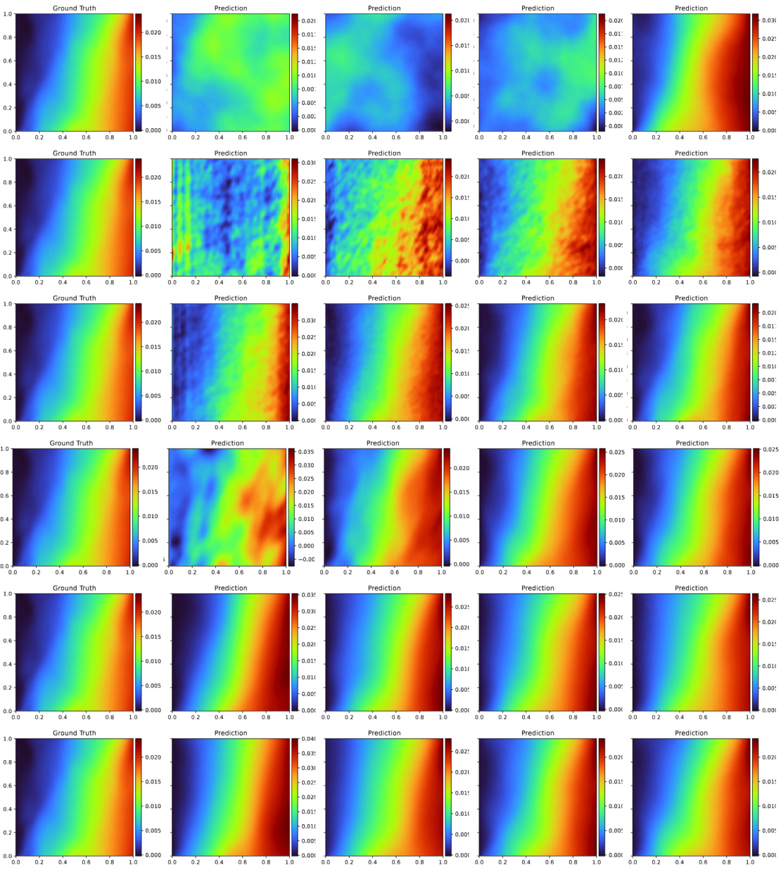
This figure compares the performance of different neural operator methods (DeepONet, FNO, DINO, and DE-DeepONet) for solving two nonlinear PDEs: hyperelasticity and Navier-Stokes. It shows the relative errors in L2 and H1 norms for solution prediction, as well as the Frobenius norm error for the prediction of the solution’s derivative with respect to the input parameters. The plots illustrate how the accuracy of each method varies with the number of training samples.

This figure compares the performance of different neural operator methods (DeepONet, FNO, DINO, DE-DeepONet) for solving two nonlinear PDEs: hyperelasticity and Navier-Stokes. It shows the relative errors in L2 and H1 norms for the solution prediction and the relative error in the Frobenius norm for the derivative prediction with respect to the input parameter. The results are presented for varying numbers of training samples, illustrating how the accuracy improves with more data, and highlighting the improved performance of DE-DeepONet.

The figure compares the performance of several neural network methods in approximating the solution and its derivative with respect to the input parameter for two different PDEs: hyperelasticity and Navier-Stokes. The results are shown for varying numbers of training samples and across three error metrics: L2 norm, H1 norm, and Frobenius norm of the Jacobian. The plots visualize the trade-off between training data size and prediction accuracy for each method.

This figure compares the performance of various neural network methods (DeepONet, FNO, DINO, and DE-DeepONet) for solving two types of PDEs: hyperelasticity and Navier-Stokes equations. It shows three error metrics (L² norm, H¹ norm, and Frobenius norm) plotted against the number of training samples. The L² and H¹ norms measure the accuracy of the solution prediction, while the Frobenius norm evaluates the accuracy of the derivative prediction. The results demonstrate the impact of training data size on the accuracy of each method and indicate which methods perform better under data scarcity.
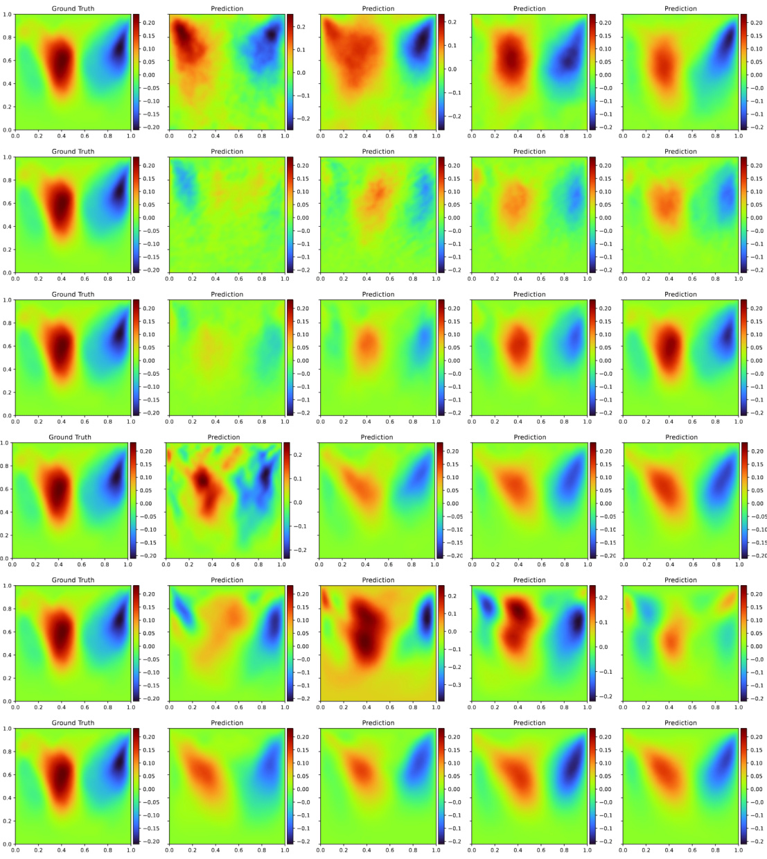
This figure compares the performance of several neural network methods (DeepONet, FNO, DINO, DE-DeepONet) on two PDE problems (hyperelasticity and Navier-Stokes) across a range of training sample sizes. It shows the relative error in three metrics: L²(Ω) norm and H¹(Ω) norm for the solution prediction, and Frobenius norm for the prediction of the Jacobian (derivative with respect to parameters). The results illustrate the impact of training sample size on accuracy and the relative effectiveness of the various neural operator methods.
More on tables

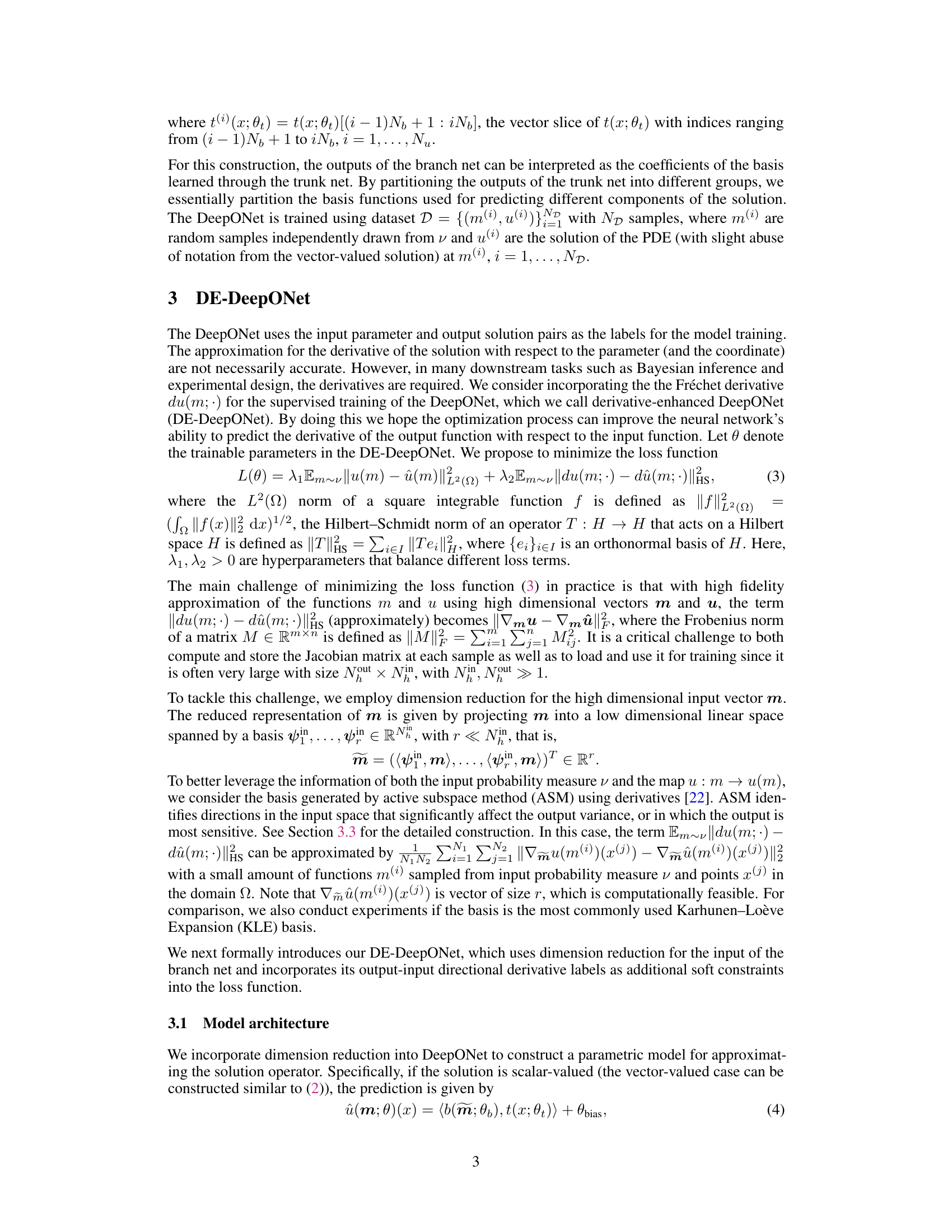
This table shows the time spent on different stages of data generation for the hyperelasticity and Navier-Stokes equations. The data generation process includes generating Gaussian random fields (GRFs), solving the PDEs using 64 processors, calculating the KLE and ASM bases using 1 and 16 processors, respectively, and generating derivative labels using 64 processors. The number of samples used is Nall = 2000, and the number of reduced basis functions is r = 16.

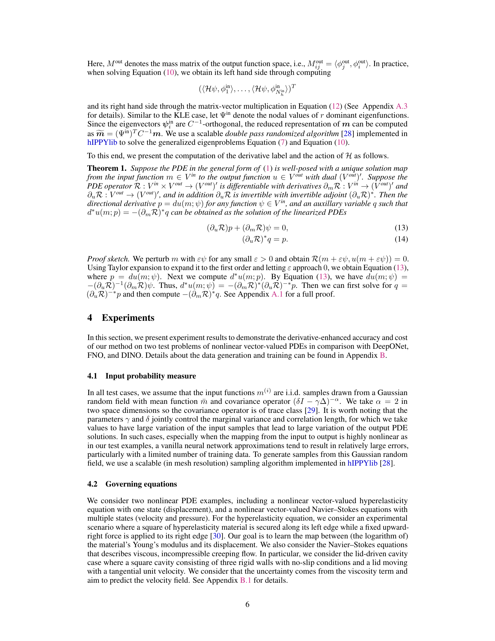
This table presents the inference time (in seconds) for five different models (DeepONet, FNO, DE-FNO, DINO, and DE-DeepONet) when evaluating 500 test samples. The inference involves calculating both the solution and its derivative (dm) in 128 random directions. The time is measured using a single GPU and a single CPU, except for DINO where it uses both a GPU and a CPU, and a separate measurement is provided using 16 CPUs for DE-DeepONet. This demonstrates the relative computational efficiency of different methods for solving PDEs.

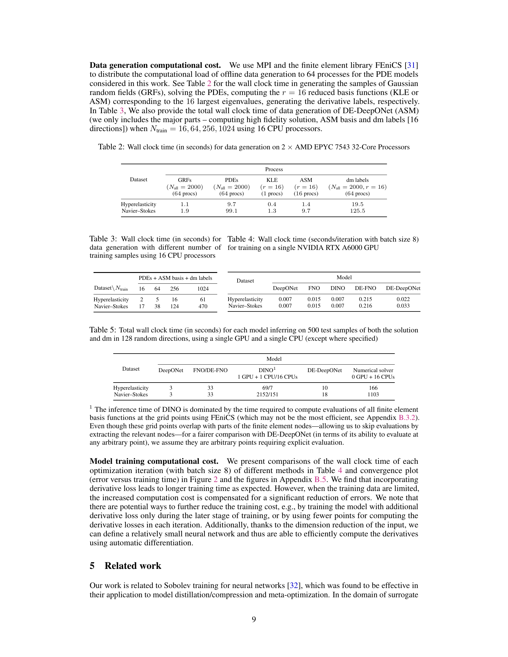
This table compares the inference time of different models (DeepONet, FNO, DE-FNO, DINO, and DE-DeepONet) on two datasets (Hyperelasticity and Navier-Stokes). The inference time is measured for 500 test samples and directional derivatives in 128 random directions. The use of a single GPU and a single CPU is consistent, except for DINO which uses 1 GPU and 1 CPU or 16 CPUs depending on the approach, and the numerical solver which uses only 16 CPUs. The table highlights the computational efficiency of different models in the context of evaluating the solutions and derivatives.

This table details the configurations used for generating the datasets employed in the paper’s experiments. It specifies the mesh resolution (64x64), the type of finite element used (CG), the polynomial degree of the finite element (deg=1 or deg=2), the number of training and testing samples (Ntrain, Ntest), the number of reduced basis functions (r), and the number of samples used for computing the ASM basis (Ngrad). Separate configurations are given for the hyperelasticity and Navier-Stokes datasets, reflecting differences in problem formulation and solution space dimensions.

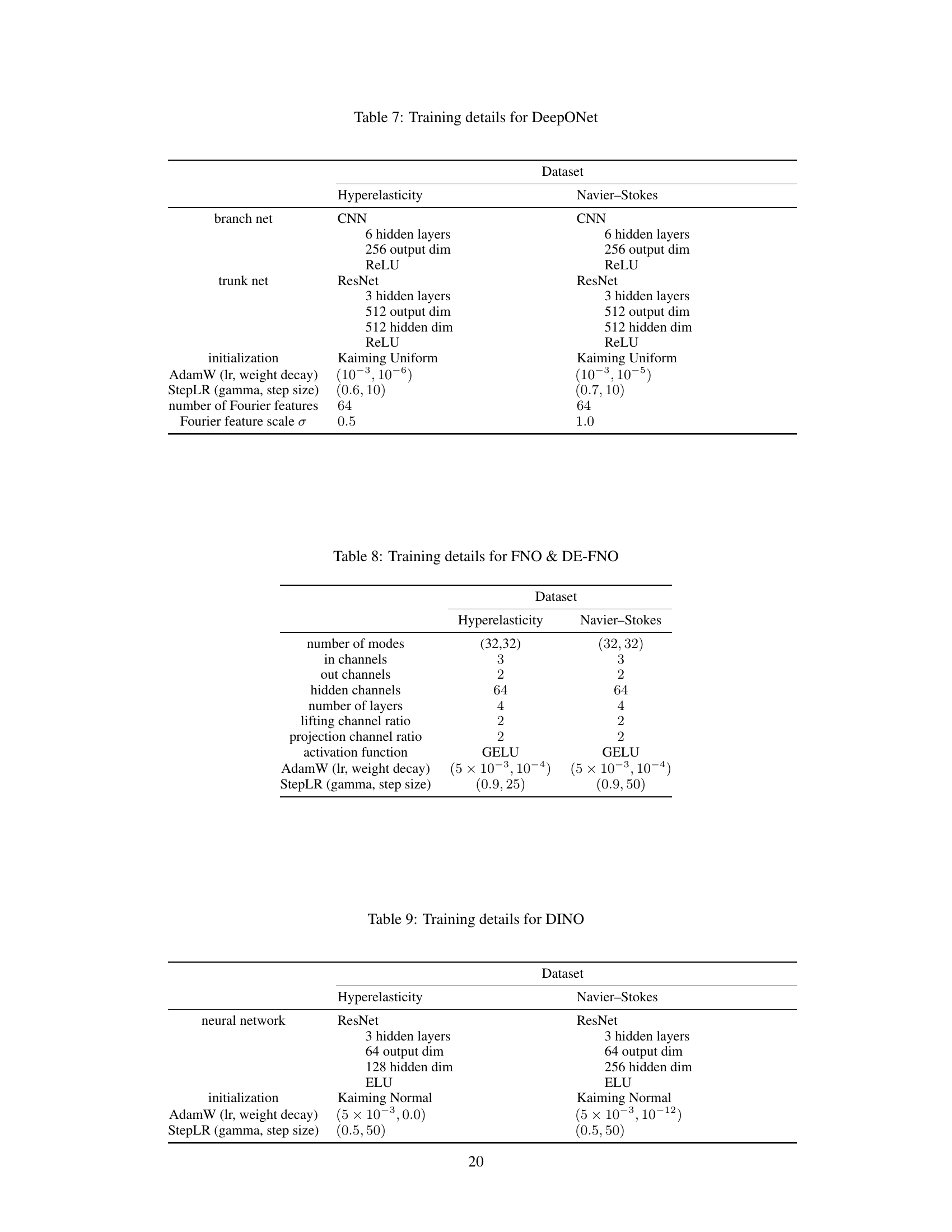
This table details the configurations used for training the DeepONet model on two datasets: Hyperelasticity and Navier-Stokes. It specifies the architecture of both the branch net and trunk net (using CNN and ResNet respectively), including the number of hidden layers, output dimensions, hidden dimensions, activation functions (ReLU), and initialization method (Kaiming Uniform). The table also provides hyperparameters for the AdamW optimizer (learning rate and weight decay), StepLR scheduler (gamma and step size), number of Fourier features, and the scale of Fourier feature embeddings (σ). The specific values of these parameters vary slightly between the Hyperelasticity and Navier-Stokes datasets.

This table details the hyperparameters used for training the Fourier Neural Operator (FNO) and the derivative-enhanced FNO (DE-FNO) models. The hyperparameters include the number of modes, input and output channels, hidden channels, number of layers, lifting and projection channel ratios, activation function, AdamW optimizer learning rate and weight decay, and StepLR scheduler parameters. Separate configurations are provided for the hyperelasticity and Navier-Stokes datasets.

This table presents the configuration of the neural network architecture (ResNet), initialization method (Kaiming Normal), optimizer (AdamW) with learning rate and weight decay, learning rate scheduler (StepLR) with gamma and step size for the hyperelasticity and Navier-Stokes datasets in the DINO model. The number of hidden layers, output dimension, and hidden dimension are also specified for both datasets.

This table details the specific hyperparameters and settings used to train the DE-DeepONet model for both the hyperelasticity and Navier-Stokes datasets. It specifies the architecture of the branch and trunk networks (both ResNet), the number of hidden layers, output dimensions, hidden dimensions, activation functions (ELU or ReLU), initialization method (Kaiming Uniform), AdamW optimizer parameters (learning rate and weight decay), whether the learning rate scheduler is disabled, the number of Fourier features used, the scale of the Fourier features (σ), and the batch size (Nbatch) used during training.

This table shows the number of trainable parameters for four different neural operator architectures (DeepONet, FNO, DINO, and DE-DeepONet) applied to two different datasets (Hyperelasticity and Navier-Stokes). It highlights the relative model complexity and provides context for the computational cost comparisons discussed in the paper. Note that DE-DeepONet uses significantly fewer parameters than FNO, suggesting a potential advantage in terms of computational efficiency.
Full paper#

