↗ OpenReview ↗ NeurIPS Homepage ↗ Chat
TL;DR#
Large language models (LLMs) show remarkable proficiency in language tasks, but their internal mechanisms are not well understood. One major challenge is understanding how LLMs use their training data statistics, which is crucial for improving model training and addressing issues like brittleness and bias. This paper attempts to demystify transformer predictions by describing how they depend on their context in terms of simple N-gram based statistics.
The authors develop a novel approach to study this statistical dependence. By analyzing how well a family of functions (based on simple N-gram statistics) approximates transformer predictions, they discover several things. This includes a simple way to detect overfitting, how transformers progress from learning simple to more complex statistical rules, and when transformer predictions tend to be approximated by N-gram rules. They found high agreement between the top-1 predictions of LLMs and N-gram rulesets, suggesting that N-gram rules can effectively explain a significant portion of LLM behavior.
Key Takeaways#
Why does it matter?#
This paper is crucial for researchers working with large language models (LLMs). It offers novel insights into how LLMs utilize training data, providing a new method to detect overfitting without holdout sets and a quantitative measure of LLM learning progress. These findings are significant for improving LLM training and understanding their behavior, opening new avenues for research in dataset curation and model interpretability.
Visual Insights#

The figure illustrates how different N-gram rules, derived from the training data and applied to a given context, produce different predictive distributions for the next token. The example shows three rules applied to the context ’the tired dog’: one using all three tokens (4-gram), one using only the first and last (3-gram), and one marginalizing over the middle token (also 3-gram). The choice of which rule best matches the transformer’s prediction is a key aspect of the paper’s methodology.

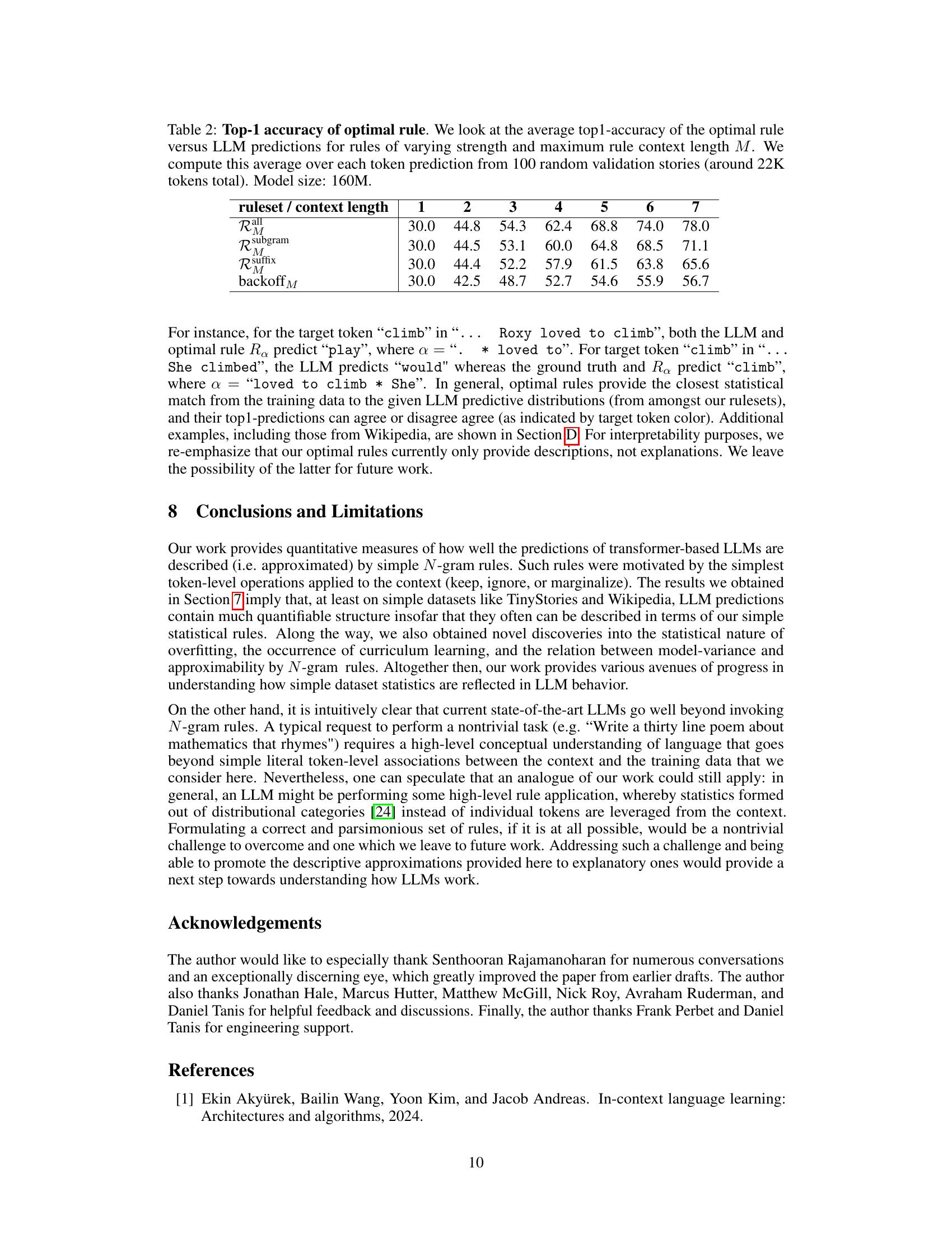
This table presents the top-1 accuracy of the optimal rule compared to the LLM predictions. The optimal rule is selected based on the minimum average distance between LLM predictions and rule predictions for rules of varying strength and context length. The results are averaged across 100 random validation stories and the model size is 160M.
In-depth insights#
Transformer Demystified#
A heading titled “Transformer Demystified” suggests an attempt to simplify and clarify the inner workings of transformer models. This could involve exploring their mathematical foundations in an accessible way, perhaps using analogies or visualizations to illustrate complex concepts like attention mechanisms and self-attention. A key aspect would likely be demystifying the ‘black box’ nature of transformers, explaining how input data is processed and how predictions are generated. The discussion might involve contrasting transformer behavior with simpler models to highlight their unique strengths and capabilities. The exploration could also examine the role of training data in shaping the model’s performance, discussing concepts like overfitting, generalization, and bias. A successful “Transformer Demystified” section would bridge the gap between theoretical understanding and practical applications, making the technology more approachable for a broader audience while still maintaining scientific rigor.
N-gram Approximation#
The concept of ‘N-gram Approximation’ in the context of large language models (LLMs) centers on using simplified N-gram statistical models to approximate the complex behavior of LLMs. This approach offers a valuable way to gain insights into how LLMs utilize their training data and make predictions. By comparing the predictions of N-gram models with those of LLMs, researchers can quantify the degree of LLM reliance on simple statistical rules derived from N-grams. The method provides a lens through which to analyze various aspects, including the detection of overfitting, the tracking of training dynamics, and a better understanding of how well LLMs can be approximated by N-gram-based rulesets. The strength of this approach lies in its simplicity and ability to unveil hidden dynamics that are otherwise difficult to observe in the intricate workings of LLMs. Limitations include the fact that N-gram models are descriptive, not explanatory and that true LLM behavior surpasses simple N-gram statistics. Despite this, N-gram approximation provides a unique tool to bridge the gap between simple statistical models and the complexity of LLMs, thereby offering crucial insights into their functioning.
LLM Learning Dynamics#
The section on “LLM Learning Dynamics” would explore how large language models (LLMs) evolve their statistical understanding of the training data during learning. Curriculum learning is a key concept, examining whether LLMs learn simpler statistical rules (e.g., based on shorter N-grams) earlier in training before progressing to more complex rules that capture longer-range dependencies. The analysis may involve tracking a measure of how well LLM predictions are approximated by rules of varying complexities (such as those based on N-gram statistics) as training progresses. The study might uncover a dynamic shift in the types of statistical rules the model relies on, potentially revealing insights into how LLMs internalize and organize their knowledge. The authors might also investigate whether the learning process displays distinct phases or patterns of rule acquisition and refinement, providing evidence for or against the notion of a learning curriculum. A key aspect to explore would be the potential correlation between the learning dynamics and other phenomena such as overfitting and generalization.
Overfitting Detection#
The proposed overfitting detection method is quite novel, leveraging the approximation of LLM predictions with N-gram rules. Instead of relying on holdout sets, it assesses the model’s ability to generalize using only training data. By analyzing the model variance across different training runs for various N-gram rules, it identifies when a model overfits. High model variance indicates overfitting, suggesting that the model is memorizing training data specifics rather than learning generalizable patterns. This is because consistent predictions (low variance) often correlate with simple statistical rules that generalize better, while inconsistent predictions (high variance) suggest over-reliance on highly specific training data features. The method’s simplicity and lack of reliance on holdout data are particularly valuable, offering a more efficient and practical approach to detecting overfitting during training.
Future Research#
Future research directions stemming from this work could involve exploring more complex rule sets beyond simple N-grams, potentially incorporating richer linguistic features or incorporating external knowledge sources. Investigating the interplay between model size, training data characteristics and the effectiveness of rule-based approximations is crucial. A deeper examination of the relationship between model variance and the applicability of N-gram rulesets is warranted. The exploration of whether similar rule-based approximations can be applied to different architectures beyond transformers and their extension to larger, more diverse datasets are important next steps. Furthermore, research is needed to bridge the gap between descriptive and explanatory rule-based models. This would entail developing methods to predict in advance when and why specific rules provide accurate approximations of LLM predictions. Finally, it would be beneficial to investigate the robustness of the proposed methods to variations in dataset biases and to different training methodologies.
More visual insights#
More on figures

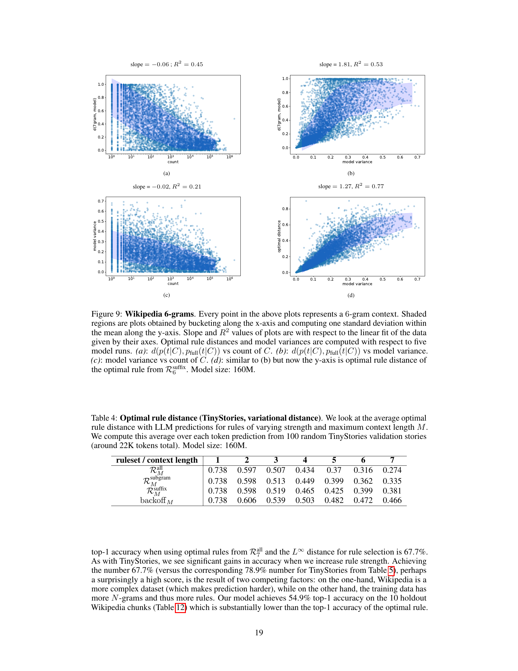
This figure visualizes the relationship between the frequency of 7-gram contexts in the TinyStories dataset, the model variance of LLM predictions for those contexts, and how well those predictions can be approximated by N-gram rules. Panel (a) shows the distance between LLM predictions and the full-context 8-gram rule versus the context’s frequency. Panel (b) shows the same distance versus model variance. Panel (c) shows model variance versus context frequency. Panel (d) shows the distance to the best-fitting N-gram rule (from a set of suffix-based rules) versus model variance. The figure demonstrates that contexts with low model variance tend to be well-approximated by N-gram rules, even when rare. This supports the paper’s approximation criterion.

This figure shows the learning dynamics of LLMs. The left panel shows that the distance between LLM predictions and the optimal rules (based on n-gram statistics) decreases as training progresses, with more complex rules being learned later in training. The central and right panels show that while the overall distance between LLM predictions and the optimal rules may plateau, the quality of the optimal rule selection increases over training as measured by top-1 accuracy relative to the ground truth.

This figure shows the training and validation loss curves for various LLMs trained on the TinyStories dataset. The models differ in their context length—the number of previous tokens they consider when predicting the next token. The full transformer model exhibits overfitting, showing a decreasing training loss but an increasing validation loss. In contrast, the models with limited context lengths show nearly identical training and validation loss curves, indicating that they do not overfit. This suggests that overfitting occurs when LLMs try to memorize long contexts instead of generalizing from shorter sub-contexts.
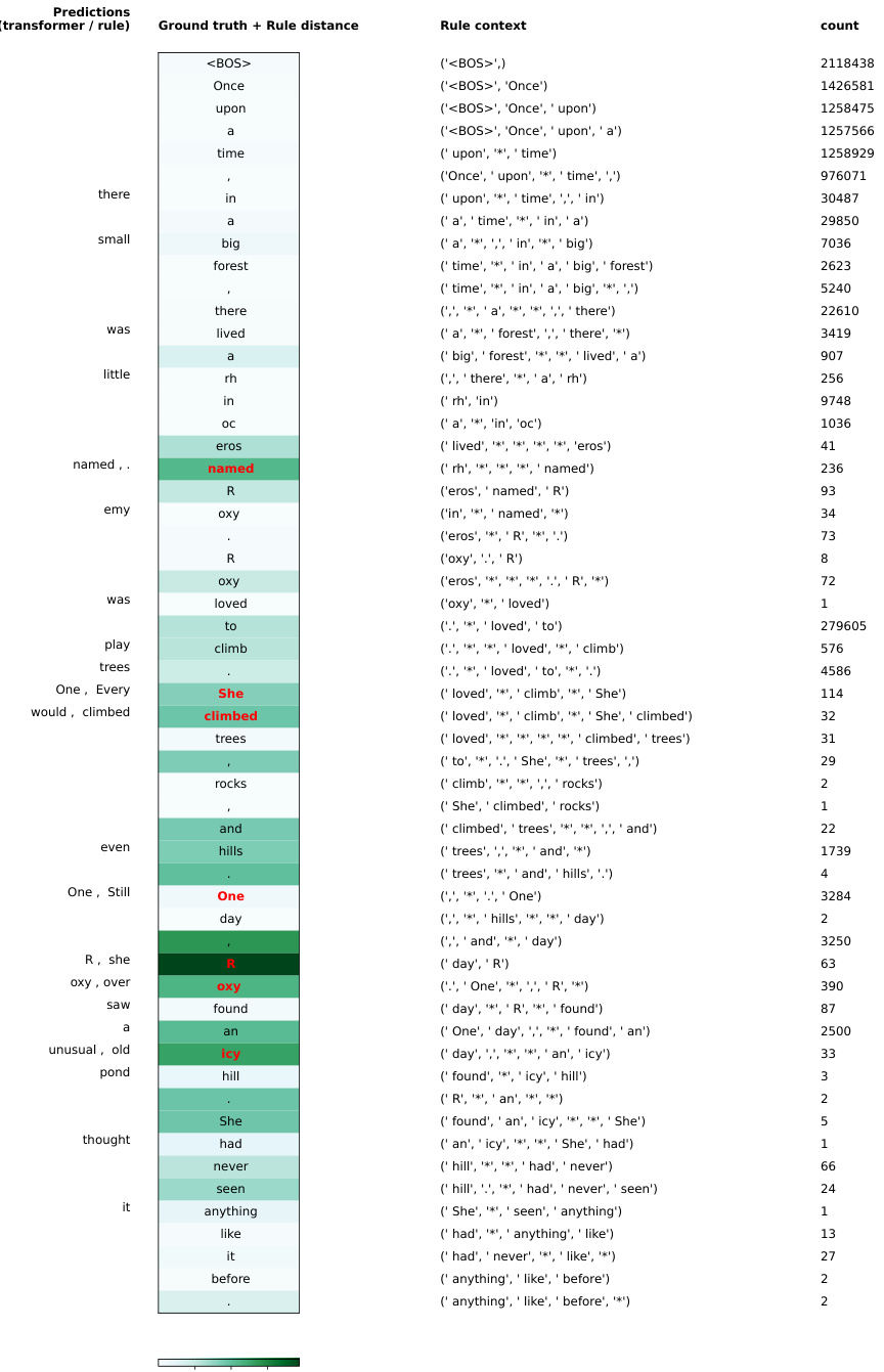
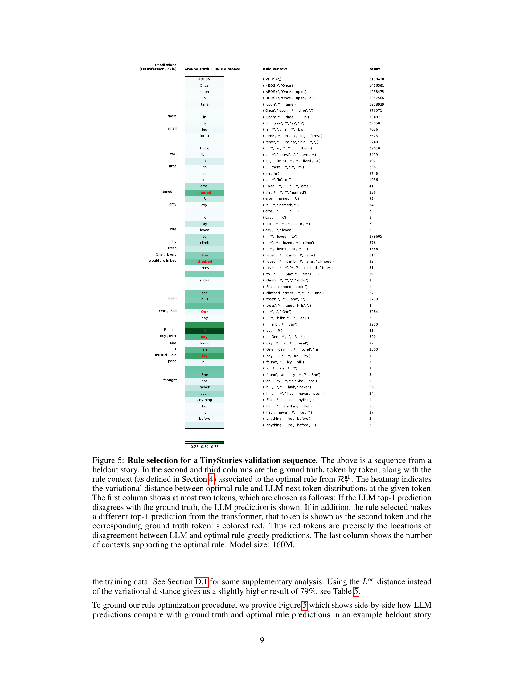
This figure shows an example of rule selection for a heldout story from the TinyStories dataset. It compares the LLM’s next-token predictions with the ground truth and optimal rule predictions, highlighting disagreements using color-coding. The heatmap visualizes the variational distance between the LLM and optimal rule distributions for each token. The context of the optimal rule and its supporting context count are also provided.

This figure compares the performance of two transformer models, one trained with full context and another trained with a context length of 1, against a bigram model on the TinyStories dataset. The x-axis represents the count of each unigram, and the y-axis represents the variational distance between the transformer model’s predictions and the bigram model’s predictions for that unigram. The scatter plot shows that as the unigram count increases, the variational distance generally decreases for both transformer models, indicating improved approximation of the bigram model by the transformers. The figure highlights the impact of context length on the ability of transformer models to learn simple bigram statistics.
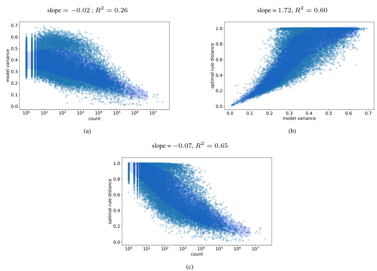
This figure visualizes the relationship between the frequency of 7-gram contexts in the training data, the variance of LLM predictions across different training runs, and how well those predictions can be approximated by N-gram rules. It shows that contexts with low variance tend to be well-approximated by rules, even if they are rare in the training data. The plots show the distances between LLM predictions and the best-fitting N-gram rule, as well as model variance, against the count of each 7-gram context in the training data.
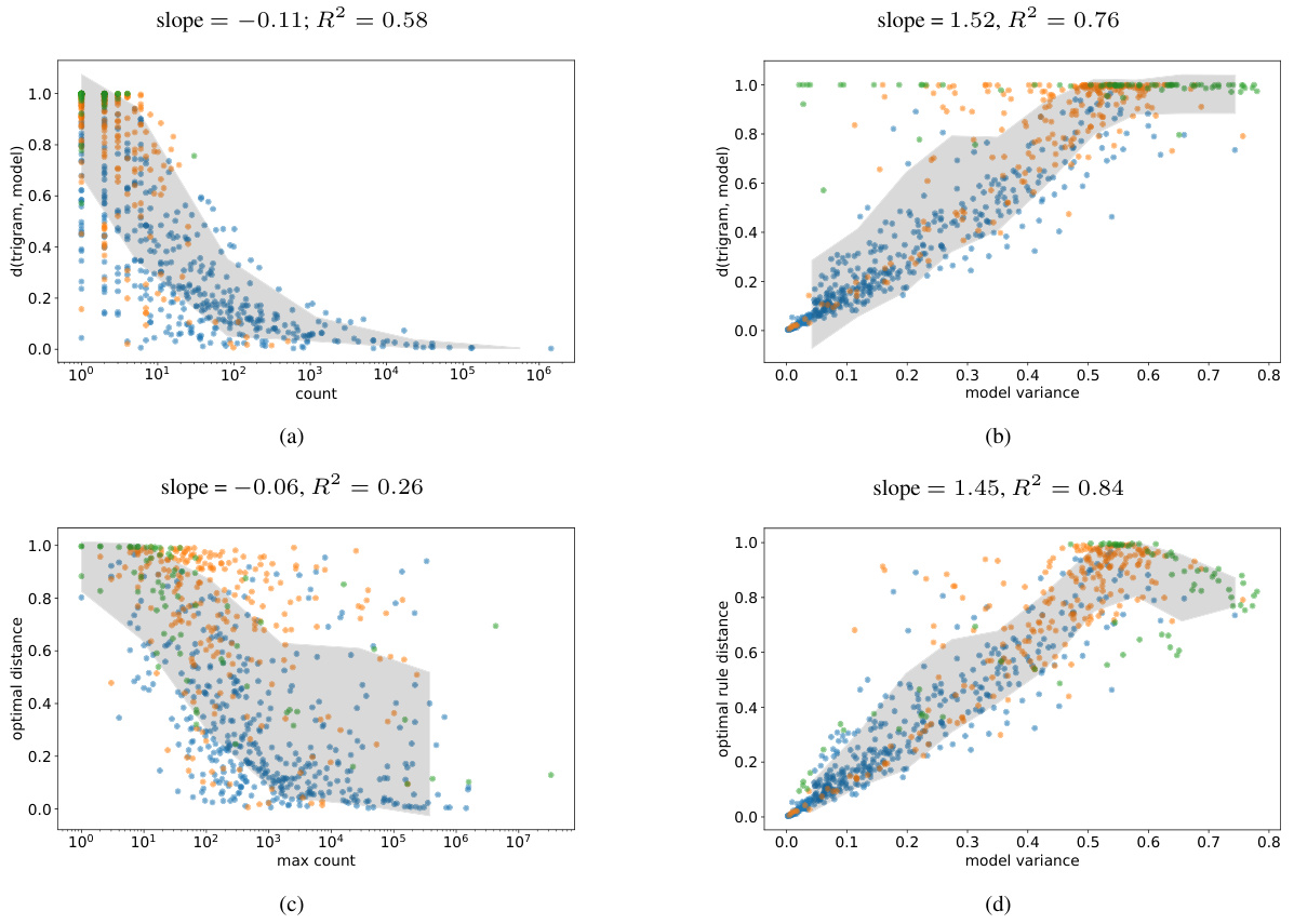
This figure visualizes the relationship between the frequency of 7-gram contexts in the training data, the variance of LLM predictions across different runs, and the distance between LLM predictions and the predictions of the best-fitting N-gram rule. It shows that contexts with low variance across runs tend to be well-approximated by N-gram rules, even when those contexts are rare in the data. The figure supports the paper’s approximation criterion, demonstrating how LLMs rely on simpler rules for low-variance predictions and leverage more complex rules for high-variance predictions.
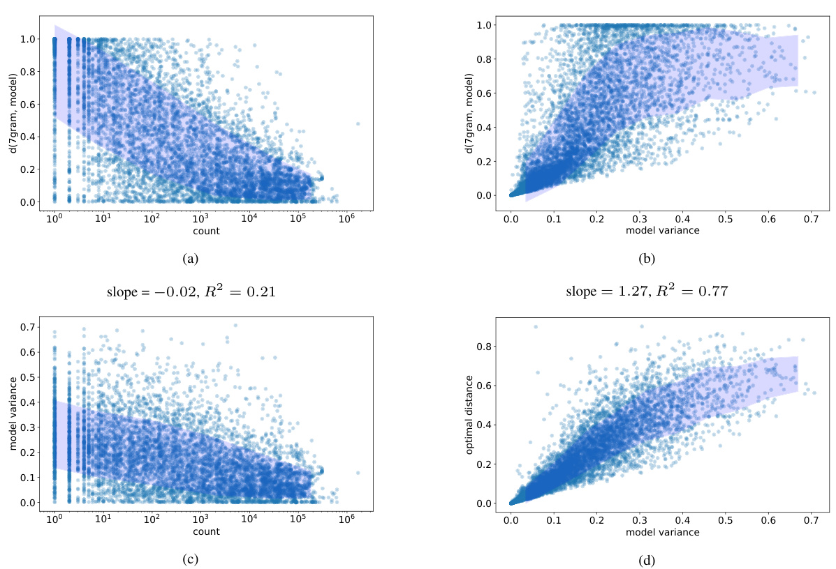
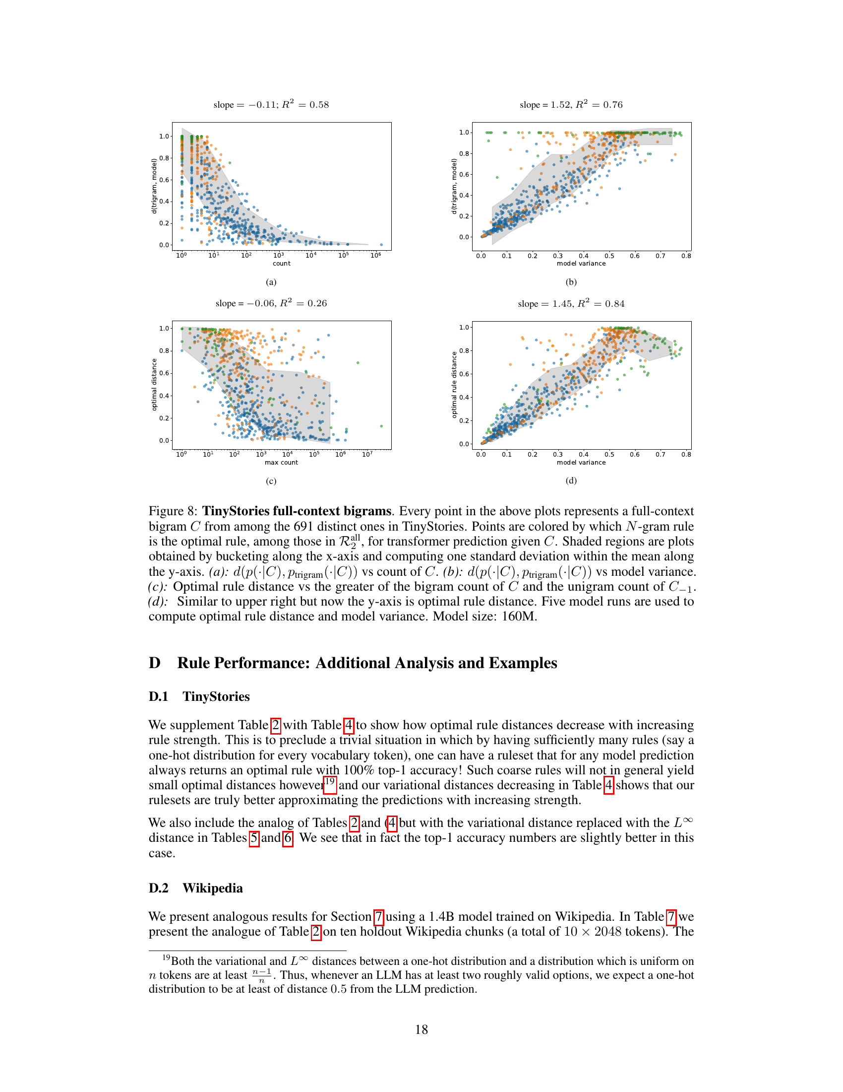
This figure visualizes the relationship between the frequency of 7-gram contexts in the training data, model variance, and the distance of LLM predictions from the full-context 8-gram rule. It shows that low model variance in LLM predictions is associated with a closer approximation to N-gram rules, particularly for higher-frequency contexts.

This figure demonstrates an example of rule selection for a held-out TinyStories sequence. It shows the ground truth tokens, the LLM’s top-1 predictions, the optimal rule’s predictions, and the variational distance between the LLM’s and optimal rule’s probability distributions for each token. Red tokens indicate disagreements between the LLM and the optimal rule’s top-1 predictions. The context used for each rule is also shown, along with the number of times that context appeared in the training data. This helps illustrate how the model’s predictions relate to simple statistical rules extracted from the training data.

This figure shows an example of rule selection for a heldout TinyStories sequence. It demonstrates how the model’s top-1 prediction compares to the ground truth and the predictions of an optimal N-gram rule. The heatmap visually represents the variational distance between the model and rule predictions for each token. Red tokens highlight discrepancies between the model’s top-1 prediction and both the ground truth and the optimal rule.

This figure shows an example of rule selection for a heldout story from the TinyStories dataset. It compares the ground truth, the LLM prediction, and the prediction of the optimal rule from the ruleset Rall. The heatmap visualizes the variational distance between the LLM and optimal rule predictions for each token. Tokens where the LLM prediction and ground truth disagree are highlighted, showing where the model and optimal rule diverge. The number of contexts supporting the optimal rule is also given, providing insights into the model’s reliance on specific contexts.

This figure shows an example of how the model selects rules for a held-out sequence from the TinyStories dataset. The heatmap visualizes the difference between the model’s prediction and the optimal rule’s prediction for each token. Red tokens highlight discrepancies between the model and the optimal rule. The context and count of supporting contexts for each rule are also provided.
More on tables

This table presents the top-1 accuracy results comparing the optimal rule’s predictions against the LLM’s predictions. The accuracy is calculated for different rule complexities (context lengths from 1 to 7) and three different rule types (all, subgram, suffix). A baseline using a simple backoff method is also included. The results are averaged across 100 validation stories, offering a comprehensive evaluation of the rule’s effectiveness in approximating LLM predictions.

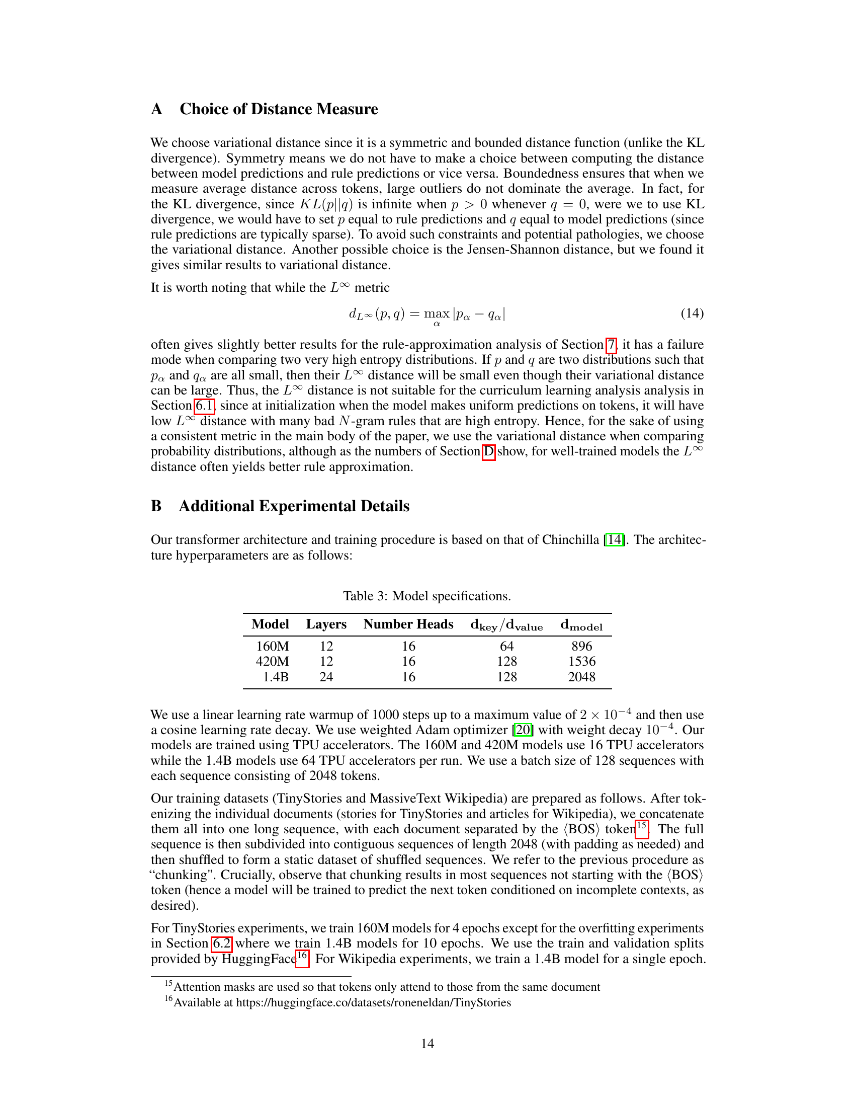
This table presents the architectural hyperparameters of the transformer models used in the experiments. It shows the number of layers, the number of attention heads, the dimension of the key/value vectors (dkey/dvalue), and the overall model dimension (dmodel) for three different model sizes: 160M, 420M, and 1.4B parameters. These specifications are based on the Chinchilla architecture.

This table shows the average optimal rule distance between the LLM predictions and the rule predictions for different rulesets (Rall, Rsubgram, Rsuffix, and backoffM) and context lengths (1-7). The optimal rule distance measures how well the LLM predictions can be approximated by the rules in each ruleset. A lower optimal rule distance indicates a better approximation. The data is from 100 random TinyStories validation stories, and the model size is 160M.

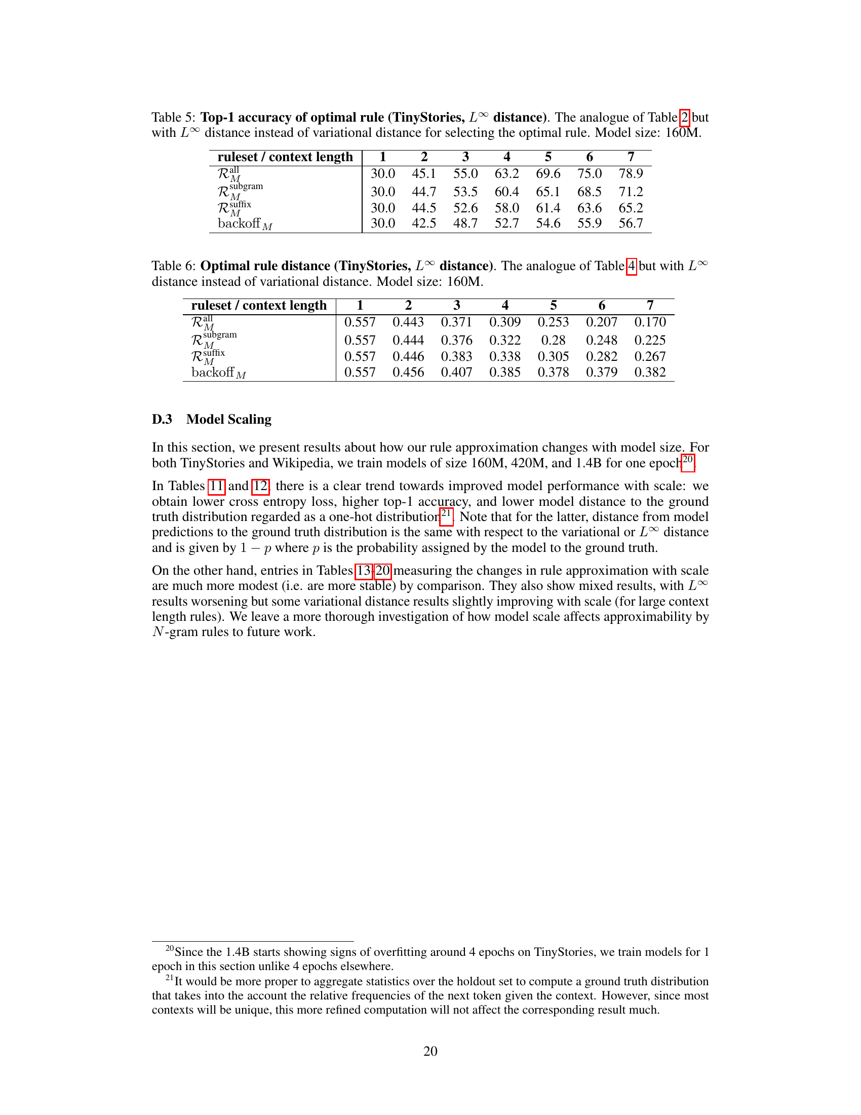
This table shows the top-1 accuracy of the optimal rule for different rulesets and context lengths, using the L∞ distance metric. It’s a comparison to Table 2, which used the variational distance. The model size used was 160M parameters. The results indicate the performance of using different N-gram rules to predict the next token in the TinyStories dataset.

This table shows the average optimal rule distance between LLM predictions and optimal rules for different rule strengths and maximum context lengths (1-7 tokens). The L∞ distance metric is used instead of the variational distance used in Table 4. The model size used is 160M. This table helps to understand how well the predictions made by the language model (LLM) can be approximated by the simple statistical rules defined in the paper, using a different distance metric than Table 4.

This table presents the top-1 accuracy results of using optimal rules to predict the next token, compared to the LLM’s predictions. It shows the average top-1 accuracy across various rule complexities (context lengths) and rule types, providing insights into how well N-gram based rules can approximate transformer predictions. The results are averaged across 100 validation stories, for a 160M parameter model.

This table shows the average optimal rule distance between the LLM predictions and the rule predictions for rules of varying strength and maximum context length, computed over each token prediction from 100 random validation stories. The model size is 160M. The table helps to understand how the approximation improves with increasing rule strength.

This table shows the top-1 accuracy of the optimal rule compared to the LLM predictions for different rulesets (Rall, Rsubgram, Rsuffix) and maximum context lengths (M=1 to 7). The accuracy is averaged over 100 random validation stories and calculated for each token. The model size used is 160M. It demonstrates how the accuracy changes as the complexity of the rule and the amount of context used increase.

This table shows the average optimal rule distance with LLM predictions for rules of varying strength and maximum context length. The L∞ distance is used instead of the variational distance. The average is computed over each token prediction from 100 random TinyStories validation stories. The model size used is 160M.

This table shows how the average cross-entropy loss, top-1 accuracy, and model distance to the ground truth change with different model sizes (160M, 420M, and 1.4B parameters) on a held-out set of 100 stories from the TinyStories dataset. The results demonstrate the impact of model size on performance metrics.

This table shows how the evaluation metrics (cross-entropy loss, top-1 accuracy, and model distance to ground truth) change with different model sizes (160M, 420M, and 1.4B) on a held-out set of 10 Wikipedia chunks. It demonstrates the scaling behavior of the model’s performance as its size increases.

This table shows the top-1 accuracy of the optimal rule for different model sizes (160M, 420M, and 1.4B parameters) and varying context lengths (1 to 7). The optimal rule is selected from the Rall ruleset using the variational distance metric. The results indicate how the top-1 accuracy of the optimal rule changes with increasing model size and context length.

This table shows how the minimum distance between an LLM’s next-token prediction and the prediction of an optimal rule varies with model size (160M, 420M, 1.4B parameters) and maximum context length (1-7 tokens). The optimal rule is selected from the set of all possible rules (Rall) based on the variational distance between the LLM and rule predictions. Lower distances indicate better approximation by the rules.

This table shows the top-1 accuracy of the optimal rule selected from the Rall ruleset using the L∞ distance metric for different model sizes (160M, 420M, and 1.4B parameters) and context lengths (1 to 7). The results indicate the performance of using simple N-gram rules to approximate the complex predictions of the transformer model. The accuracy increases with increasing context length and model size, suggesting that larger models with more context are better able to capture the statistical properties of the data and make better predictions.

This table shows the top-1 accuracy of the optimal rule compared to the LLM predictions for different rule complexities (context lengths) and different types of rulesets. The results are averaged over 100 validation stories with a total of approximately 22,000 tokens. The model size used is 160M parameters.

This table shows the top-1 accuracy of the optimal rule on the Wikipedia dataset using the L∞ distance for rule selection. The results are presented for varying context lengths (1-7) and for three different rule sets (Rall, Rsubgram, and Rsuffix). A backoff method is included for comparison. The model size used was 1.4B. The average is computed across each token prediction from 10 heldout sequences, each 2048 tokens long.

This table shows how the average optimal rule distance between LLM predictions and optimal rules changes with different model sizes (160M, 420M, 1.4B parameters) and rule context lengths (1-7 tokens). The optimal rules are selected using the variational distance. Lower values indicate better approximation of LLM predictions by the N-gram rules.

This table presents the top-1 accuracy of the optimal rule, comparing it against LLM predictions. The optimal rule is selected using the L∞ distance. The results are averaged over each token prediction from 10 heldout Wikipedia sequences, each consisting of 2048 tokens. The model size used is 1.4B. Different rule strengths and maximum context lengths (M) are considered.

This table shows how the optimal rule distance (using the L∞ metric) changes with different model sizes (160M, 420M, 1.4B) and rule context lengths (1-7). The optimal rule is selected from the RMall ruleset. Lower values indicate better approximation of LLM predictions by the rules.
Full paper#
