Exploiting Representation Curvature for Boundary Detection in Time Series

↗ OpenReview ↗ NeurIPS Homepage ↗ Chat

TL;DR

#

Key Takeaways

#

Why does it matter?

#

This paper is important because it introduces a novel approach to boundary detection in time series that is superior to existing methods, particularly for gradual changes. This is highly relevant to many fields that deal with time series data, such as climate science, finance, and healthcare. It could lead to better insights from time-series data, improve preprocessing steps, and enable the development of more accurate and efficient algorithms.

Visual Insights

#

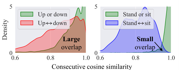
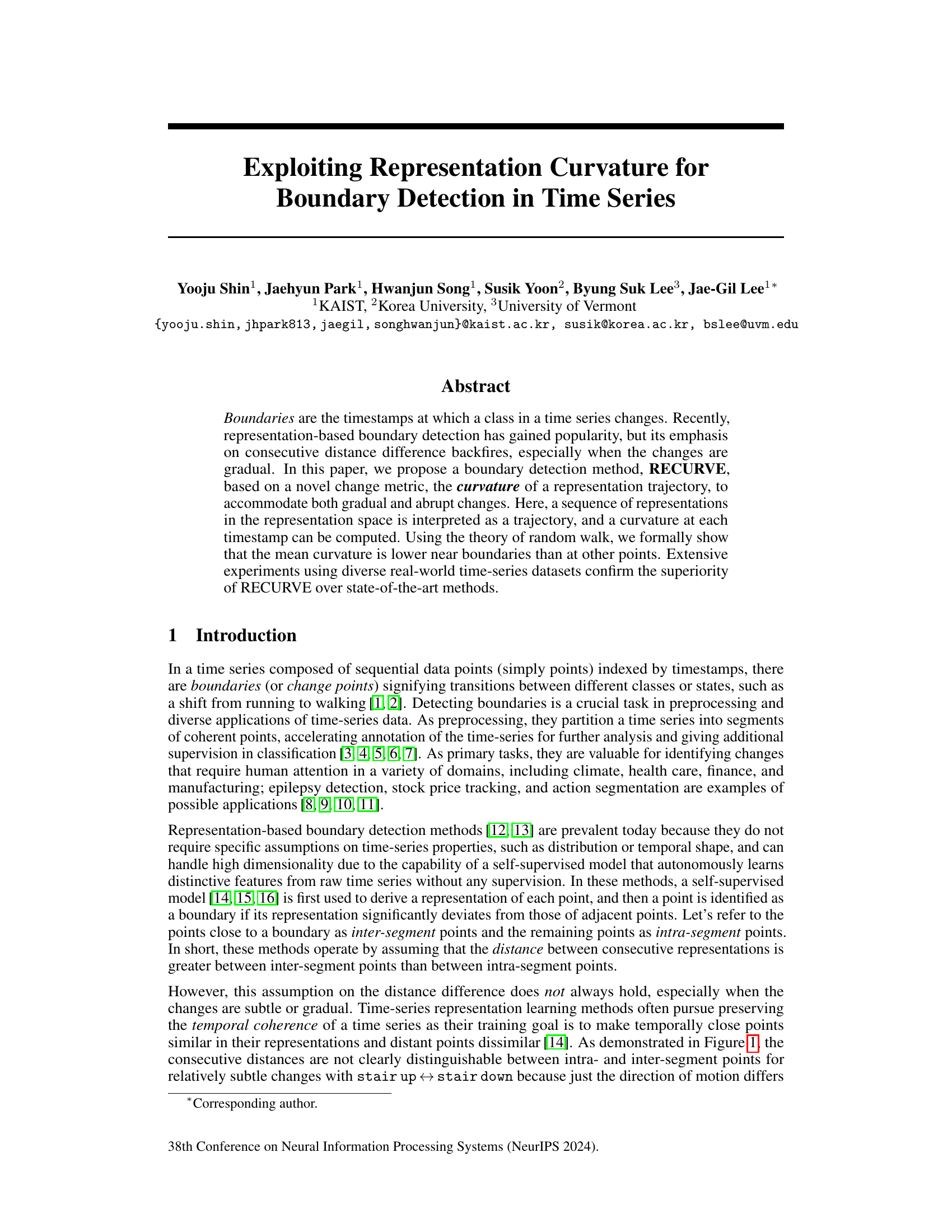
This figure shows the distribution of consecutive cosine similarity between representation vectors in the HAPT dataset. It compares intra-segment points (points within the same activity segment) and inter-segment points (points at transitions between activity segments). The goal is to illustrate the limitations of using consecutive distance differences to identify boundaries, especially when changes are subtle. The figure shows that for gradual changes (e.g., ‘up or down’), the distributions overlap significantly, making it difficult to distinguish between intra- and inter-segment points based solely on distance. However, for abrupt changes (e.g., ‘stand ↔ sit’), the distributions overlap less.

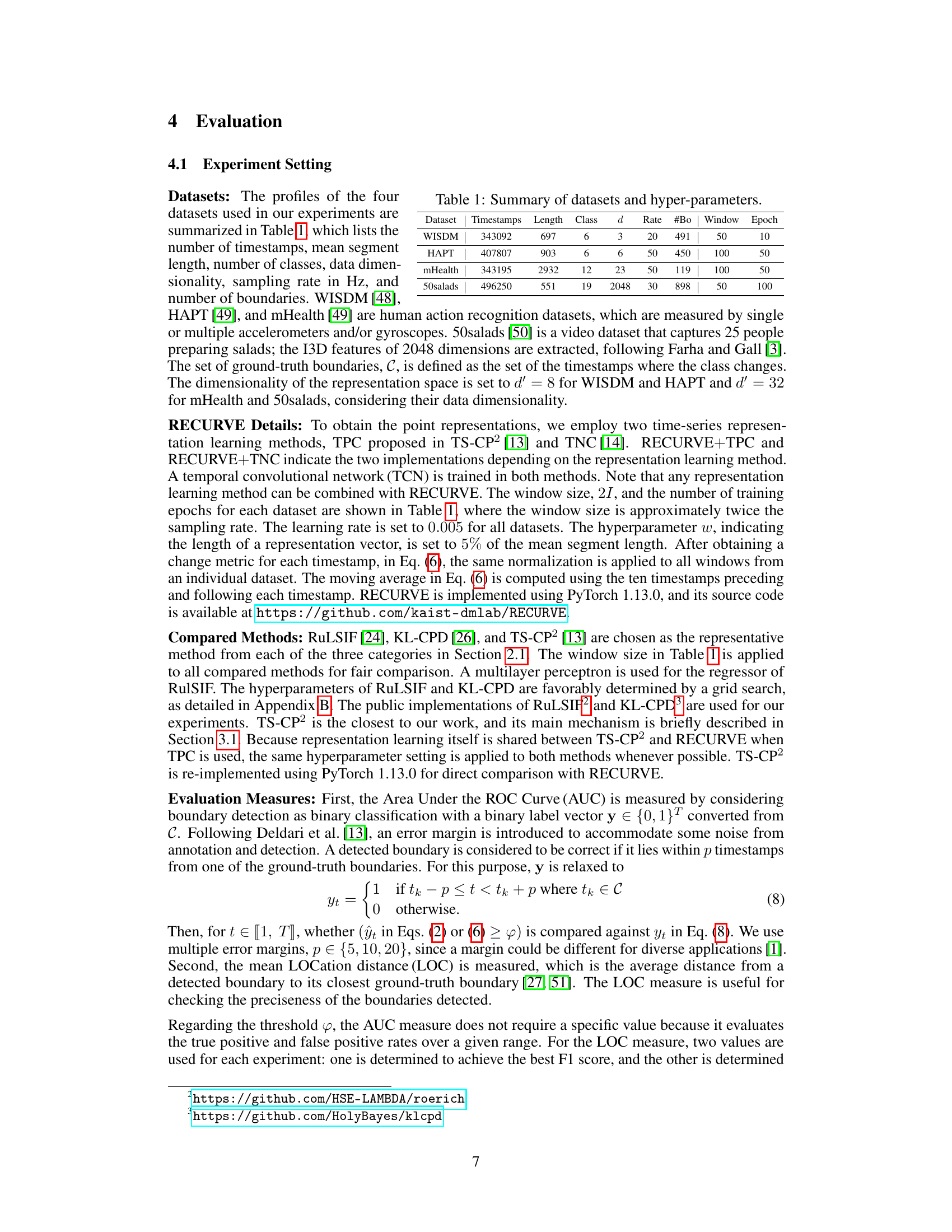
This table summarizes the characteristics of four datasets used in the experiments. For each dataset, it provides the number of timestamps, the average length of segments between boundaries, the number of classes, the dimensionality of the data, the sampling rate in Hz, the number of boundaries, the size of the sliding window used for representation learning, and the number of training epochs.

In-depth insights

#

Curvature-Based Change

#

The concept of ‘Curvature-Based Change’ offers a novel approach to boundary detection in time series analysis by shifting focus from the traditional reliance on consecutive distance differences between data points to the curvature of the representation trajectory in a feature space. This approach is particularly beneficial for handling gradual changes, which often obscure clear distance-based distinctions between segments. By interpreting a sequence of representations as a trajectory, the method calculates curvature at each timestamp. Lower curvature values are indicative of boundaries, signifying a less sharp change in direction of the trajectory and a transition between different classes. This is formally supported by a theoretical analysis, demonstrating that mean curvature is lower near boundaries due to the confinement of representation points within class-specific regions. The method’s strength lies in its ability to effectively detect boundaries regardless of the abruptness of change, overcoming a significant limitation of traditional representation-based methods. The use of curvature enhances the detection of subtle changes that are often missed by distance-based approaches, demonstrating its effectiveness across diverse real-world datasets and its robustness to inherent ambiguities in various time-series data.

Representation Trajectories

#

Representation trajectories offer a powerful lens for analyzing time series data. By embedding each time point into a feature space, we create a trajectory that captures the temporal evolution of the data. The curvature of this trajectory, rather than simple distances between consecutive points, becomes a crucial metric for detecting boundaries or change points. This approach elegantly handles both gradual and abrupt changes, a significant improvement over traditional methods. Analyzing the curvature provides a way to detect subtle shifts, not just large jumps in the data’s characteristics. The formal analysis grounding this technique in random walks is noteworthy, providing a theoretical underpinning for its effectiveness. The intuitive notion of a trajectory turning sharply near a boundary, visually depicted as high curvature, contrasts with the limitations of distance-based methods that can struggle to differentiate intra-segment and inter-segment distances in subtle transitions. This approach promises improvements in robustness and accuracy, especially when dealing with noisy or high-dimensional time series.

Boundary Detection

#

Boundary detection in time series aims to identify timestamps marking transitions between classes or states. Traditional methods often rely on consecutive distance differences in representation space, which can be unreliable, especially with gradual changes. RECURVE, a novel method, leverages representation trajectory curvature, a more robust metric capturing directional changes regardless of the transition’s abruptness. The method’s effectiveness stems from the formal proof that lower mean curvature indicates boundaries. Extensive empirical validation across diverse real-world datasets demonstrates RECURVE’s superiority over existing state-of-the-art methods, especially for subtle, gradual changes, highlighting its adaptability and potential for broader application in various time-series analysis domains.

RECURVE Algorithm

#

The RECURVE algorithm is a novel approach to boundary detection in time series data, shifting focus from consecutive distance differences to the curvature of representation trajectories. Instead of relying on simple distance metrics, which can be misleading for gradual changes, RECURVE leverages the inherent geometric properties of representation space. By treating sequential data representations as a trajectory, it calculates curvature at each point, showing that lower curvature indicates boundaries regardless of whether changes are abrupt or gradual. This is theoretically grounded, proven using random walk theory, and empirically validated across diverse real-world datasets. The algorithm’s simplicity and efficiency, combined with its ability to use any time-series representation learning method, make it a strong contender in boundary detection, demonstrating consistent improvements over state-of-the-art techniques.

Gradual Change Handling

#

Many time-series boundary detection methods struggle with gradual changes, often relying on consecutive distance differences between representations. This approach falters when transitions are subtle, as the distance metric may not reliably distinguish between intra- and inter-segment points. A more robust method is needed to capture gradual shifts effectively. The curvature-based approach in RECURVE offers an improvement because it measures the rate of directional change in the representation trajectory. This metric is sensitive to subtle changes in direction, even when the magnitude of change is small, allowing for detection of gradual boundaries that might otherwise be missed. Recurve’s use of curvature directly addresses the limitations of distance-based methods in handling gradual changes. This makes it a more reliable approach for detecting boundaries, especially when there is a lack of significant instantaneous differences between consecutive data points. The formal proof showing lower mean curvature near boundaries further supports the effectiveness of RECURVE’s strategy. This theoretical foundation, combined with empirical results, validates its superiority over traditional distance-based boundary detection methods in handling gradual transitions within time-series data.

More visual insights

#

More on figures

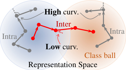
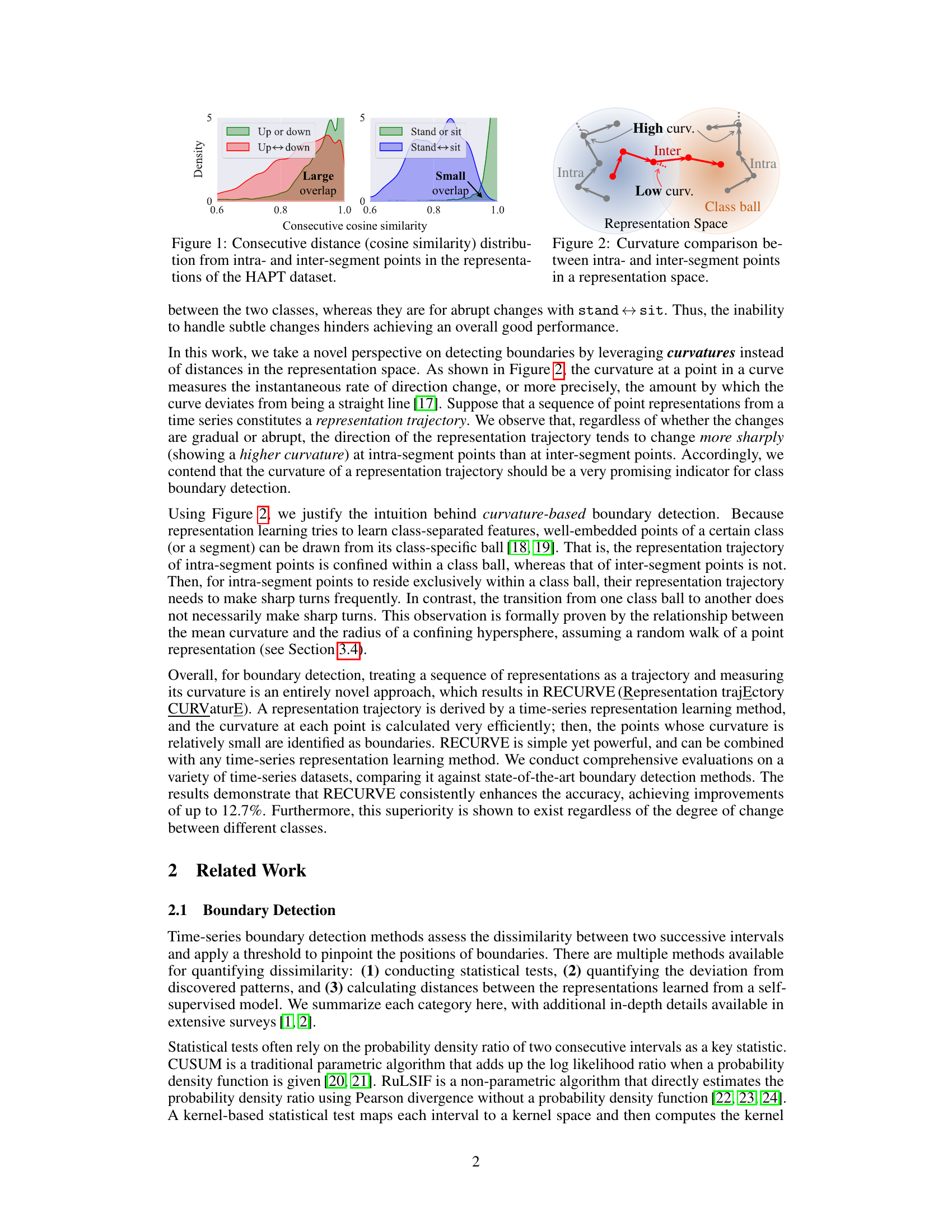
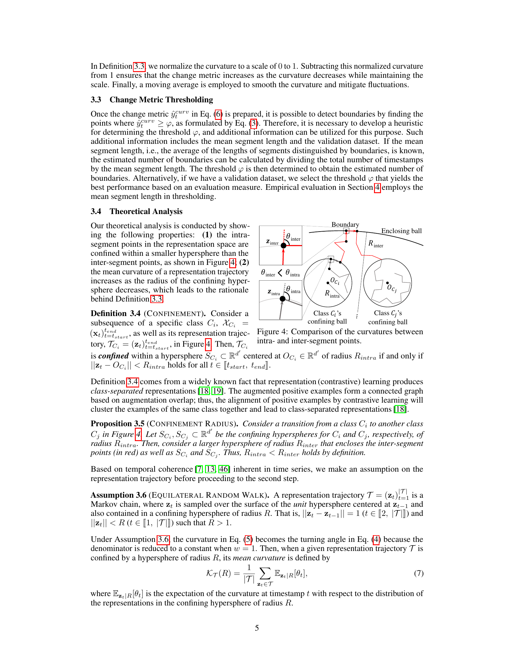
This figure illustrates the concept of confinement in the representation space. Intra-segment points (those belonging to the same class) tend to cluster tightly together within a small hypersphere (the blue circle), while inter-segment points (transitions between classes) are located in the space between hyperspheres (the orange circle). The curvature of the trajectory representing the sequence of points is higher for intra-segment points because the trajectory needs to make sharp turns to stay within the confines of the small hypersphere. In contrast, inter-segment points have a lower curvature, as they transition between hyperspheres with less sharp turns. The figure visually reinforces the core idea that curvature can be used as an effective change metric for boundary detection.

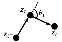
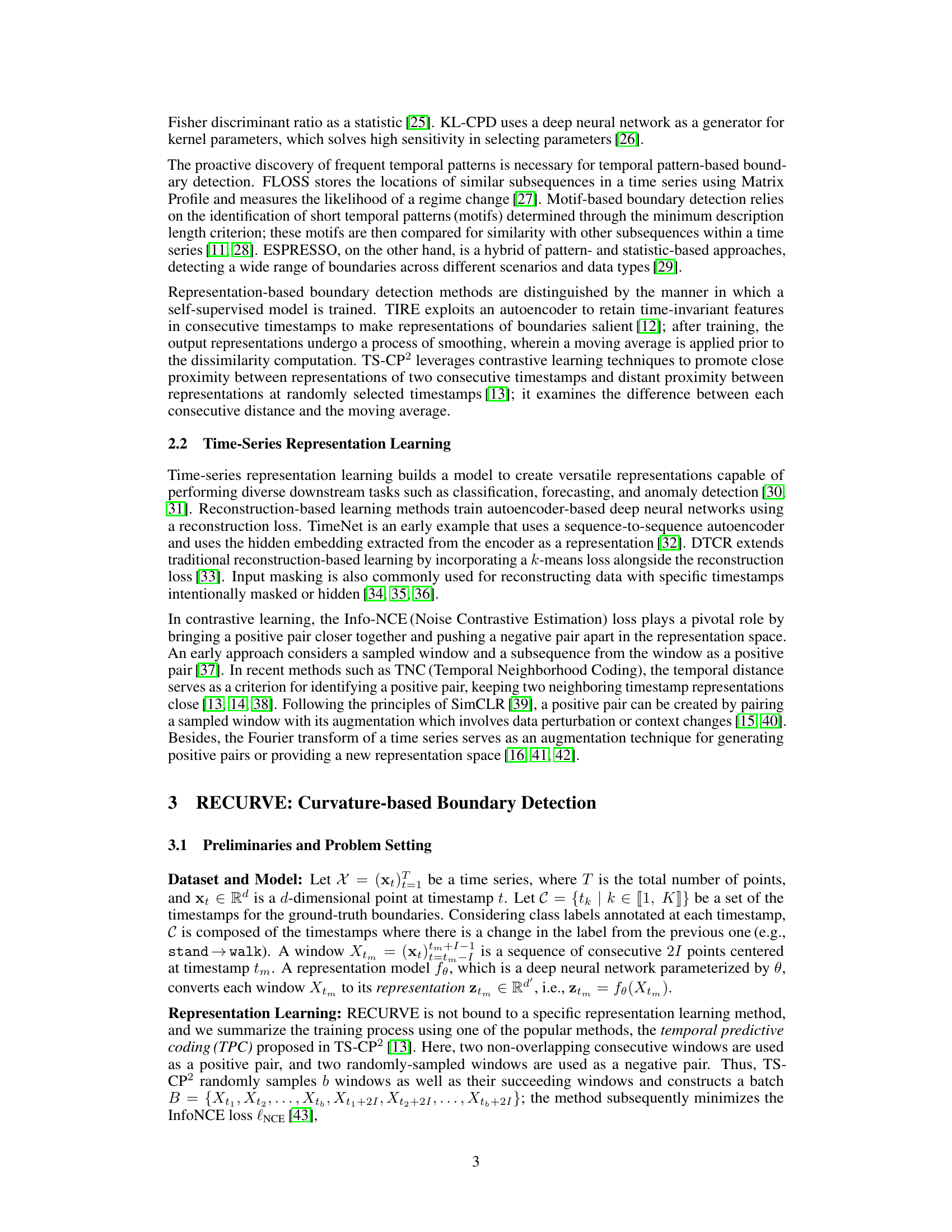
This figure shows three points in a representation trajectory (zt−,zt,zt+) at consecutive timestamps. The curvature at point zt is defined as the rate of change of direction between the two vectors (zt−−zt) and (zt+−zt). The angle θt represents this change of direction, which is used to calculate the curvature.

This figure illustrates the concept behind curvature-based boundary detection. It shows that intra-segment points (within a single class) in the representation space tend to be clustered within a smaller hypersphere (Sc;), while inter-segment points (transitioning between classes) lie in a larger hypersphere. The smaller radius of the intra-segment hypersphere implies that the trajectory of representations for intra-segment points tends to curve more sharply than for inter-segment points. This difference in curvature is used to identify boundaries.

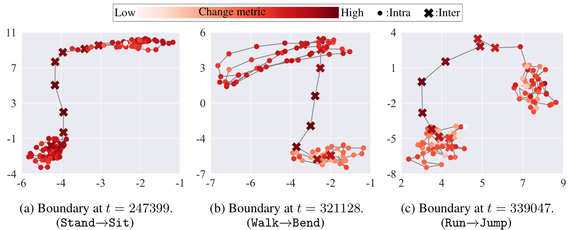
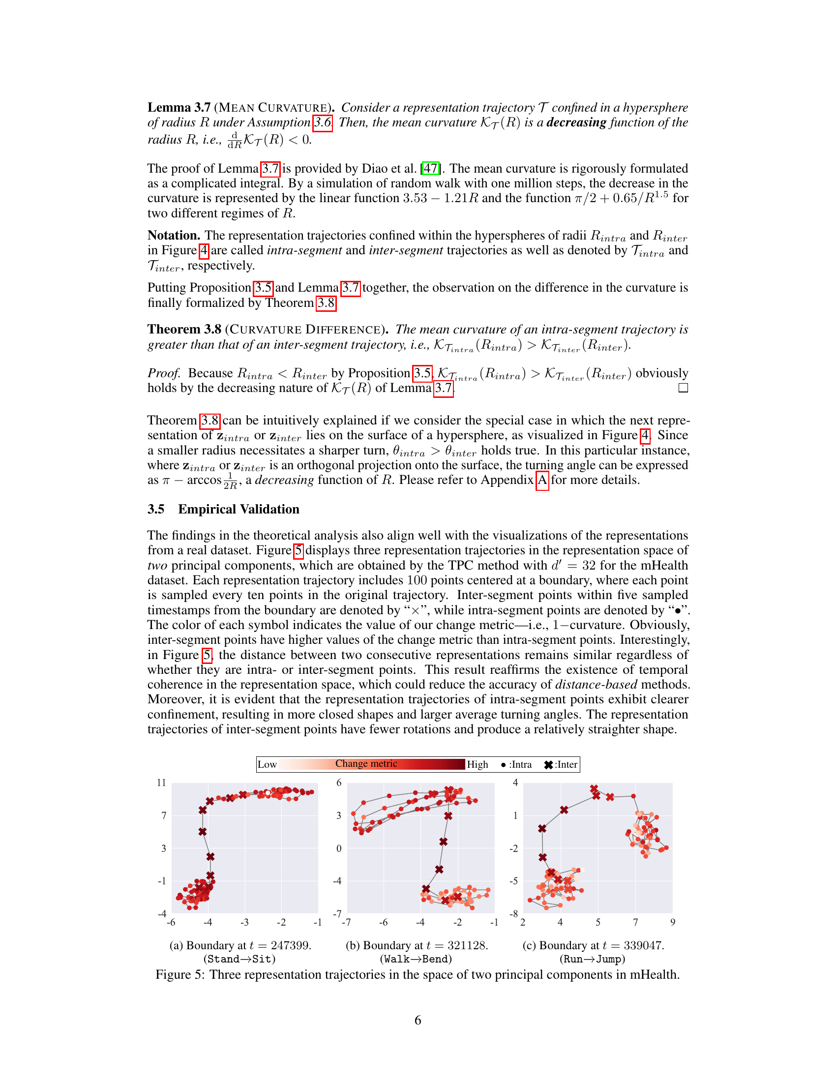
This figure visualizes three representation trajectories from the mHealth dataset projected onto the space of two principal components. Each trajectory contains 100 points sampled from the original trajectory, centered on a boundary. Inter-segment points (within five timestamps of the boundary) are marked with ‘x’, while intra-segment points are represented by ‘•’. The color intensity of each point corresponds to its change metric value (1 - curvature). The visualization aims to show how curvature can differentiate intra- and inter-segment points, even when the consecutive distances between them remain similar. Intra-segment trajectories exhibit tighter confinement with sharper turns (higher curvature), compared to straighter inter-segment trajectories.

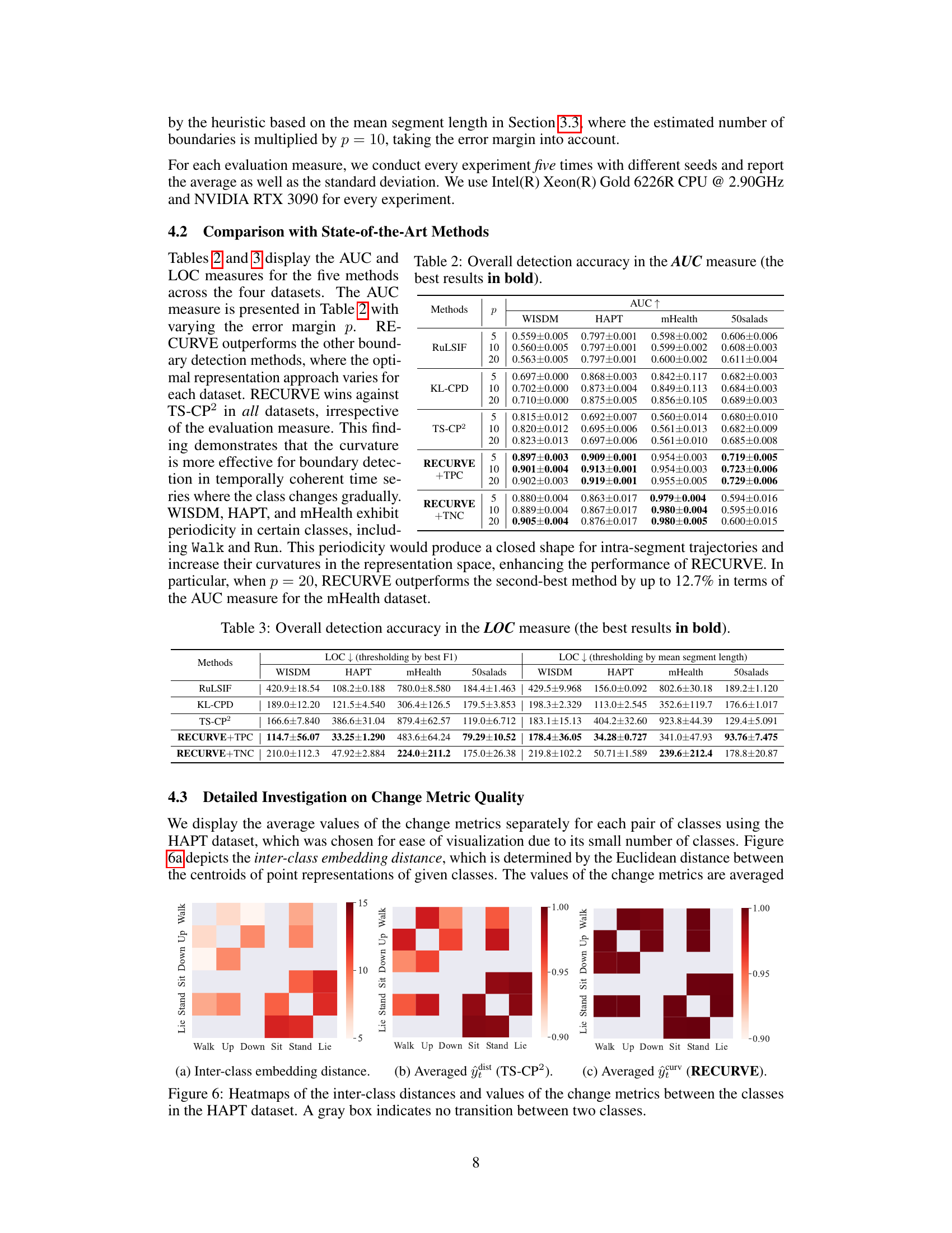
This figure compares three different ways of measuring changes between classes in the HAPT dataset. The first heatmap shows the inter-class embedding distance, which is a measure of the distance between the average representations of different classes. The second heatmap shows the averaged change metric ŷdist from the TS-CP2 method, which measures the dissimilarity between successive time intervals. The third heatmap shows the averaged change metric ŷcurv from the RECURVE method, which measures the curvature of the representation trajectory. The figure illustrates that RECURVE is better at capturing changes between classes, even when those changes are gradual, than the other methods.

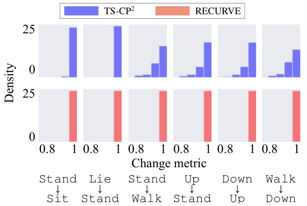
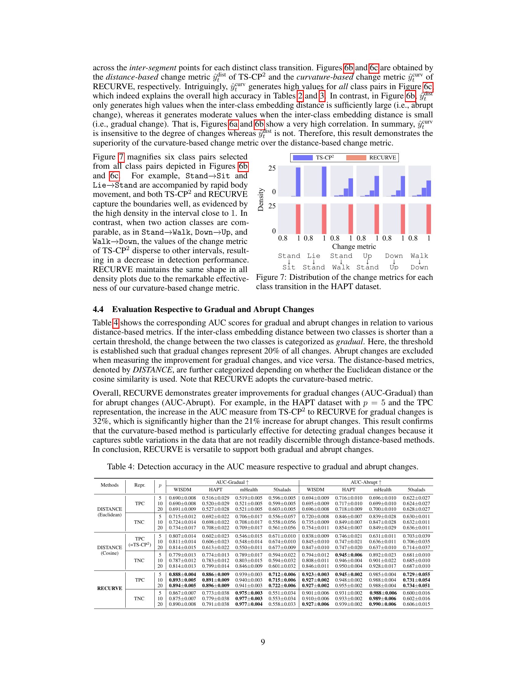
This figure compares the distribution of change metrics generated by TS-CP2 and RECURVE for six different class transitions in the HAPT dataset. The x-axis represents the change metric values (from 0.8 to 1), and the y-axis shows the density of those values. The figure visually demonstrates that RECURVE consistently produces higher change metric values across all transitions compared to TS-CP2, indicating its superior ability to capture both gradual and abrupt changes.

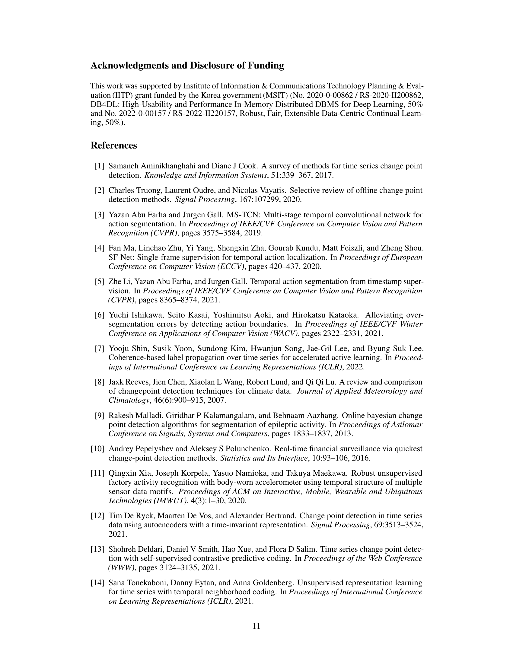
This figure visualizes the change metric scores for both TS-CP2 and RECURVE methods on the HAPT dataset. The x-axis represents timestamps, and the y-axis represents the change metric score (normalized between 0 and 1). The gray shaded regions indicate the ground truth inter-segment points (i.e., transitions between activity classes). RECURVE demonstrates clearer and more consistent identification of inter-segment points compared to TS-CP2, highlighting its superior performance in boundary detection.

More on tables

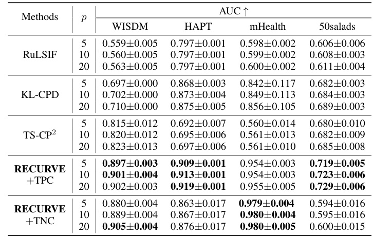
This table presents the Area Under the ROC Curve (AUC) scores for five different boundary detection methods (RuLSIF, KL-CPD, TS-CP2, RECURVE+TPC, RECURVE+TNC) across four datasets (WISDM, HAPT, mHealth, 50salads). The AUC is calculated with three different error margins (p = 5, 10, 20), representing the tolerance for error in boundary detection. The best performing method for each dataset and error margin is highlighted in bold.

This table presents the Area Under the ROC Curve (AUC) values for five different boundary detection methods across four datasets. The AUC is a common metric for evaluating the performance of binary classification. Results are shown for different error margins (p=5, 10, 20) to account for noise in the data and varying tolerances for boundary detection. The best performing method for each dataset and error margin is highlighted in bold.

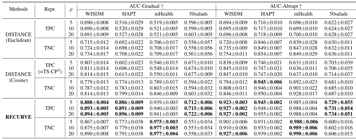
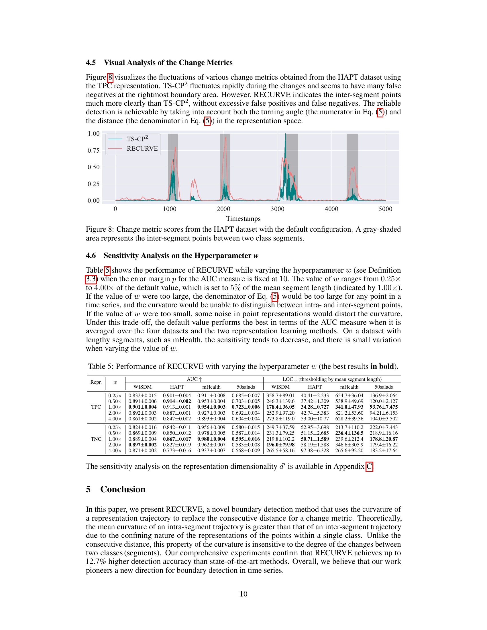
This table presents the Area Under the ROC Curve (AUC) scores for five different boundary detection methods across four datasets. The AUC is a common metric for evaluating the performance of binary classification, here measuring the ability of each method to correctly identify boundaries (change points) in time series data. The results are shown for different error margins (p = 5, 10, 20), reflecting varying levels of tolerance for slight mismatches in boundary location. The table highlights the superior performance of RECURVE compared to state-of-the-art methods in all datasets and error margin settings.

This table presents the AUC (Area Under the ROC Curve) scores for five different boundary detection methods (RuLSIF, KL-CPD, TS-CP2, RECURVE+TPC, RECURVE+TNC) across four datasets (WISDM, HAPT, mHealth, 50salads). The AUC is a measure of the ability of a classifier to distinguish between classes, with higher scores indicating better performance. Results are shown for three different error margins (p = 5, 10, 20), representing the tolerance for errors in boundary detection. The best performing method for each dataset and error margin is highlighted in bold.

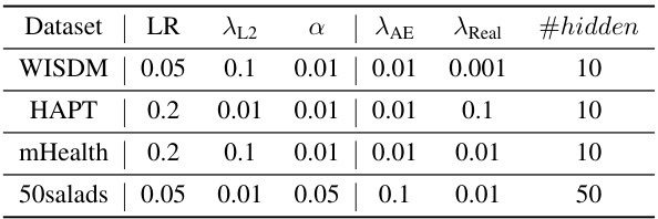
This table summarizes the characteristics of the four datasets used in the experiments, including the number of timestamps, mean segment length, number of classes, dimensionality of the data, sampling rate, and number of boundaries. It also lists the hyperparameters used for each dataset, such as window size and number of epochs. These hyperparameters are used for the representation learning method.

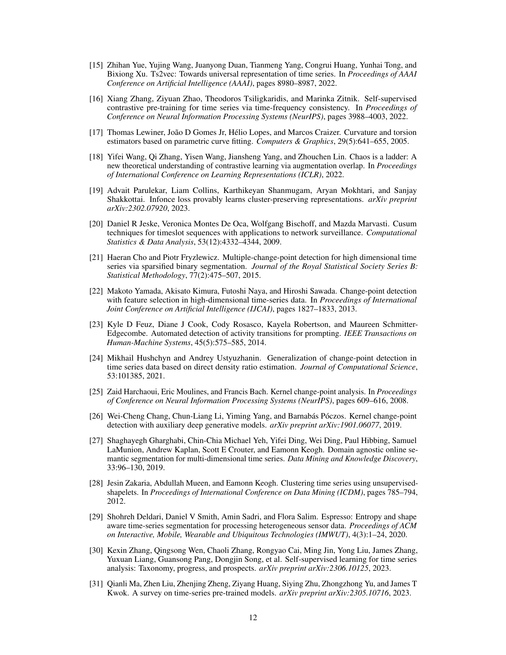
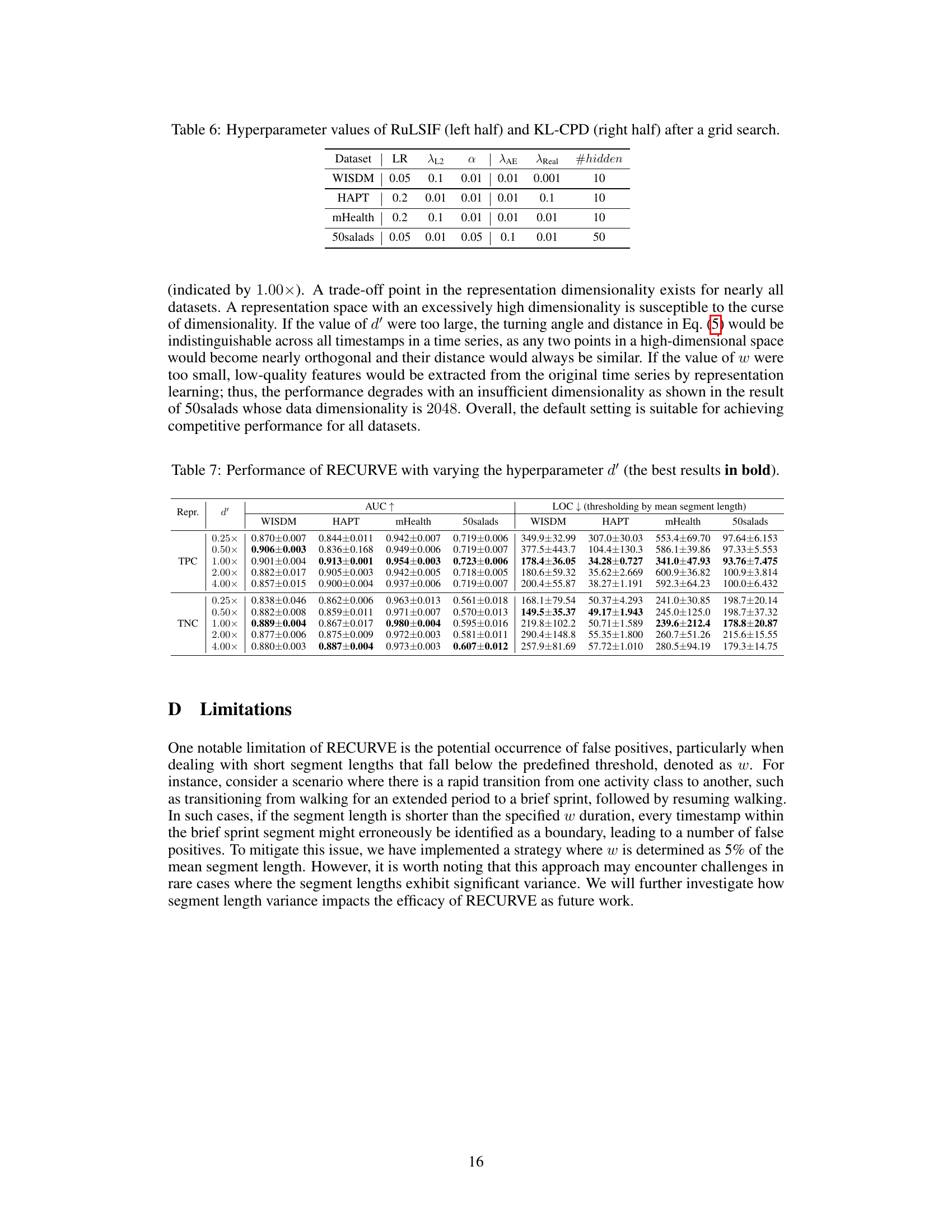
This table presents the results of an experiment that investigated the effect of varying the representation dimensionality (d’) on the performance of the RECURVE algorithm. The experiment was conducted using four different datasets (WISDM, HAPT, mHealth, and 50Salads), two different representation learning methods (TPC and TNC), and different values of d’ (0.25x, 0.50x, 1.00x, 2.00x, and 4.00x of the default value). The performance is measured using two metrics: AUC (Area Under the ROC Curve), and LOC (mean LOCation distance). For each combination of dataset, representation learning method, and d’, the table shows the mean and standard deviation of the AUC and LOC values obtained from five independent trials.

Full paper

#