↗ OpenReview ↗ NeurIPS Homepage ↗ Chat
TL;DR#
Many real-world datasets exhibit underlying symmetries which, if leveraged, can significantly improve machine learning model performance. However, identifying these symmetries often proves challenging, especially when they are not easily expressible using pre-defined mathematical groups. Existing methods often rely on explicit knowledge or are limited to simpler transformations.
This paper introduces a novel algorithm that learns continuous symmetries from data without making strong assumptions about the form of the symmetry. It uses Neural Ordinary Differential Equations (Neural ODEs) to model one-parameter groups and a novel validity score to guide the learning process. The validity score assesses how well a transformation preserves data properties relevant to a specific task. The approach demonstrates effectiveness in discovering both affine and non-affine symmetries, showcasing its advantage over existing methods on image data and partial differential equations (PDEs).
Key Takeaways#
Why does it matter?#
This paper is important because it presents a novel method for learning continuous symmetries from data, addressing a critical limitation in current machine learning techniques. It introduces a fully differentiable validity score, enabling effective searches for innate data symmetries, and demonstrates its effectiveness on image data and PDEs. This opens exciting avenues for improving model efficiency, generalization, and interpretability, which are highly sought after in the AI community. Its minimal inductive bias extends beyond common Lie group symmetries, offering broader applicability.
Visual Insights#

This figure demonstrates examples of learned symmetries using the proposed method. (a) shows vector fields, where V3 represents a learned rotational symmetry and V7 is not a symmetry. (b) displays transformed CIFAR-10 images using learned generators to illustrate the learned transformations in image data. (c) shows the transformation of PDEs (Kuramoto-Sivashinsky equation), specifically time translation and Galilean boost, highlighting the applicability of the method to different data types.
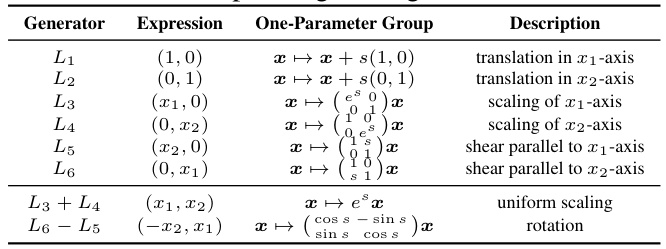
This table lists the six infinitesimal generators of the Affine group Aff(2), which are used to parameterize affine transformations in two dimensions. Each generator represents a specific type of transformation (translation along the x or y axis, scaling along the x or y axis, or shearing). The table shows the expression for each generator, the resulting one-parameter group of transformations it produces, and a short description of each transformation.
In-depth insights#
Symmetry Learning#
Symmetry learning, a subfield of machine learning, aims to leverage the inherent symmetries within data to improve model efficiency and generalization. Traditional methods often rely on pre-defined symmetries, limiting their applicability. However, recent research focuses on data-driven symmetry learning, where symmetries are learned directly from the data. This approach offers flexibility, enabling the discovery of non-linear and complex symmetries. Neural Ordinary Differential Equations (NODEs) have emerged as a powerful tool in this area, allowing continuous transformations to be learned. Validity scores, which measure how much a transformation violates the data’s underlying structure, are essential for guiding the learning process. Combining NODEs with validity scores and appropriate regularization techniques enables effective learning of continuous symmetries. The learned symmetries can then be leveraged for data augmentation and improved model performance. This approach presents significant promise for diverse applications, such as image classification and solving partial differential equations. Future work should explore the scalability and generalization abilities across different data modalities.
Neural ODE Flow#
The concept of “Neural ODE Flow” suggests a framework where neural ordinary differential equations (ODEs) are used to model the flow of data or information within a system. This approach leverages the power of ODEs to capture continuous transformations and dynamics, unlike discrete-time models that might miss crucial information. By learning the parameters of the ODE, one can model complex, continuous-time processes with a neural network. This is particularly relevant in scenarios with data that exhibit continuous symmetries or smoothly varying patterns, such as image transformations or the evolution of physical systems. A key advantage is the ability to backpropagate through the ODE solver to perform gradient-based learning, enabling end-to-end training of the entire system, including the ODE flow. However, using this approach may introduce computational challenges related to the ODE integration process. Efficient and accurate numerical ODE solvers are crucial for practical implementation, and approximations or specific solvers may need to be employed depending on the specific application. Furthermore, carefully designing the neural network architecture and the ODE model itself is important for successful training and generalization, requiring consideration of factors like stability and the trade-off between expressiveness and computational cost. Despite these potential challenges, the combination of continuous flows and deep learning offers a very powerful mechanism for modeling data.
Validity Score Design#
The effectiveness of the proposed symmetry learning algorithm hinges on the validity score design. A well-designed validity score must be differentiable and easily computable to enable efficient gradient-based optimization of the infinitesimal generators. The choice of the validity score is crucial as it determines how the algorithm assesses whether a transformation preserves the essential structure of the data for the given task. For instance, in image classification, a validity score based on the cosine similarity between feature vectors before and after transformation ensures invariance to certain image transformations. The use of pre-trained feature extractors for this purpose is a key element that simplifies the measurement of the validity score. For PDEs, a numerical error based validity score is more appropriate, ensuring that the transformed data still satisfies the governing equations with minimal changes. In both scenarios, the validity score is designed to penalize transformations that distort the essential properties of the data relevant to the task, guiding the optimization process towards symmetries that are beneficial to model performance. The sensitivity and computational efficiency of the validity score directly influence the success of the symmetry learning process, highlighting the significance of its design.
Augmentation Impact#
The augmentation impact section would likely explore how leveraging learned symmetries for data augmentation affects model performance. Key aspects to analyze would include comparisons against standard augmentation techniques (like random cropping or flipping) and the impact of varying the quantity and quality of generated augmentations. The results might show improved accuracy, particularly with limited training data. Another important point would be the generalizability of the augmentation strategy across different model architectures and datasets. For image classification, it might showcase that data augmentation using the learned symmetries produces more robust and generalized models, achieving better performance on unseen data. For PDEs, it would likely illustrate the ability of the method to successfully augment data that represents complex systems and demonstrate improvements in the neural operators’ performance and training efficiency. The analysis could also quantify the benefit of approximate symmetries compared to focusing solely on exact symmetries, highlighting situations where approximate augmentations provide substantial improvements. Overall, this section would demonstrate the efficacy of data augmentation via learned symmetries and provide a detailed quantitative analysis of this impact on model performance.
Future of Symmetries#
The “Future of Symmetries” in machine learning and scientific computing is bright, promising more efficient and generalizable models. Current methods often rely on predefined symmetries or learn them in a limited, data-driven way. Future research should focus on more flexible and robust approaches that can discover and leverage symmetries inherent in complex, high-dimensional data without strong inductive biases. This might involve exploring novel mathematical frameworks, beyond Lie groups, and developing algorithms capable of handling nonlinear and approximate symmetries. A deeper understanding of the relationship between symmetries and model interpretability is also crucial. This could involve developing methods that explicitly exploit symmetry to create more explainable and trustworthy AI systems. Furthermore, research should investigate how symmetries can be effectively incorporated into different learning paradigms, such as reinforcement learning and generative models, to improve their performance and capabilities. Ultimately, a unified theoretical framework that connects symmetries, data distributions, and model architectures is a long-term goal. This framework will enable the development of AI systems that are not only more powerful, but also more transparent and reliable.
More visual insights#
More on figures

This figure illustrates a one-parameter group generated by a vector field V. A point x0 is transported along the vector field by time s, resulting in a new point φs(x0). The curve represents the flow, showcasing how the transformation changes over time.

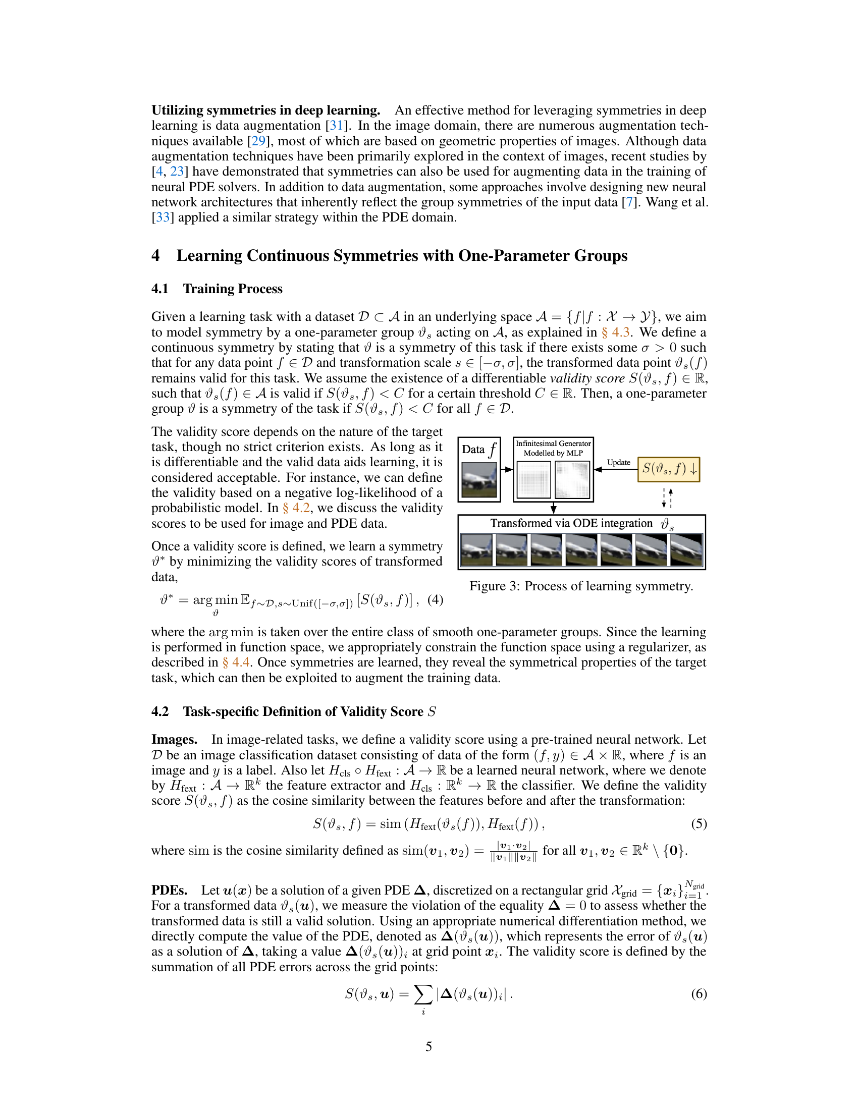
This figure illustrates the process of learning continuous symmetries using Neural ODE. The input is a data point, f, which is then transformed via ODE integration using a learned infinitesimal generator (modeled by an MLP). The transformed data point is denoted as vs(f). A validity score, S(vs, f), measures how well the transformation preserves the desired invariance for the task at hand, and this score is used to update the infinitesimal generator via backpropagation. This process aims to learn a symmetry where the validity score remains low.

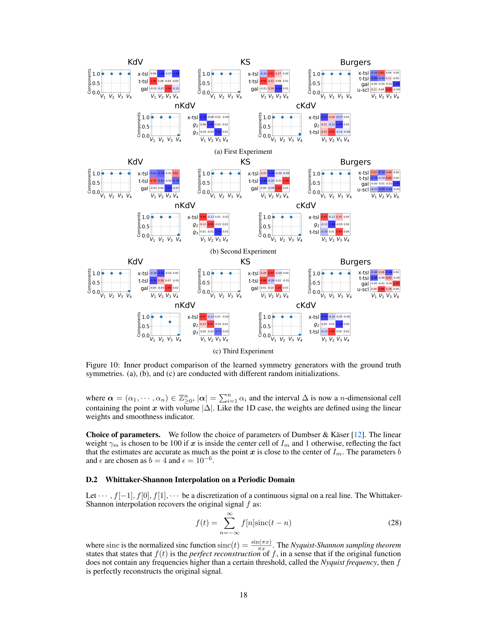
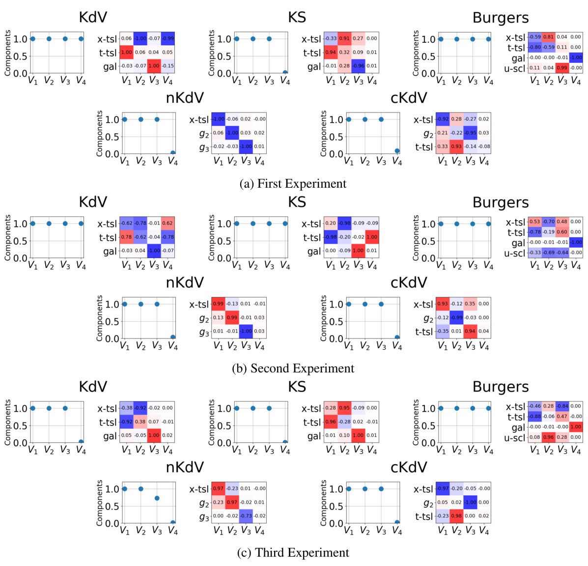
This figure compares the inner products of learned non-affine symmetry generators with their ground truth counterparts for four PDEs (KdV, KS, nKdV, and cKdV). Each subplot represents a PDE. The heatmap shows the inner product between each learned generator (V1-V4) and the ground truth symmetries (x-tsl: space translation, t-tsl: time translation, gal: Galilean boost, u-scl: u-axis scaling). A high inner product (blue) indicates a strong alignment between the learned and ground truth symmetries, showing the success of the method in identifying symmetries from data, even non-affine ones.

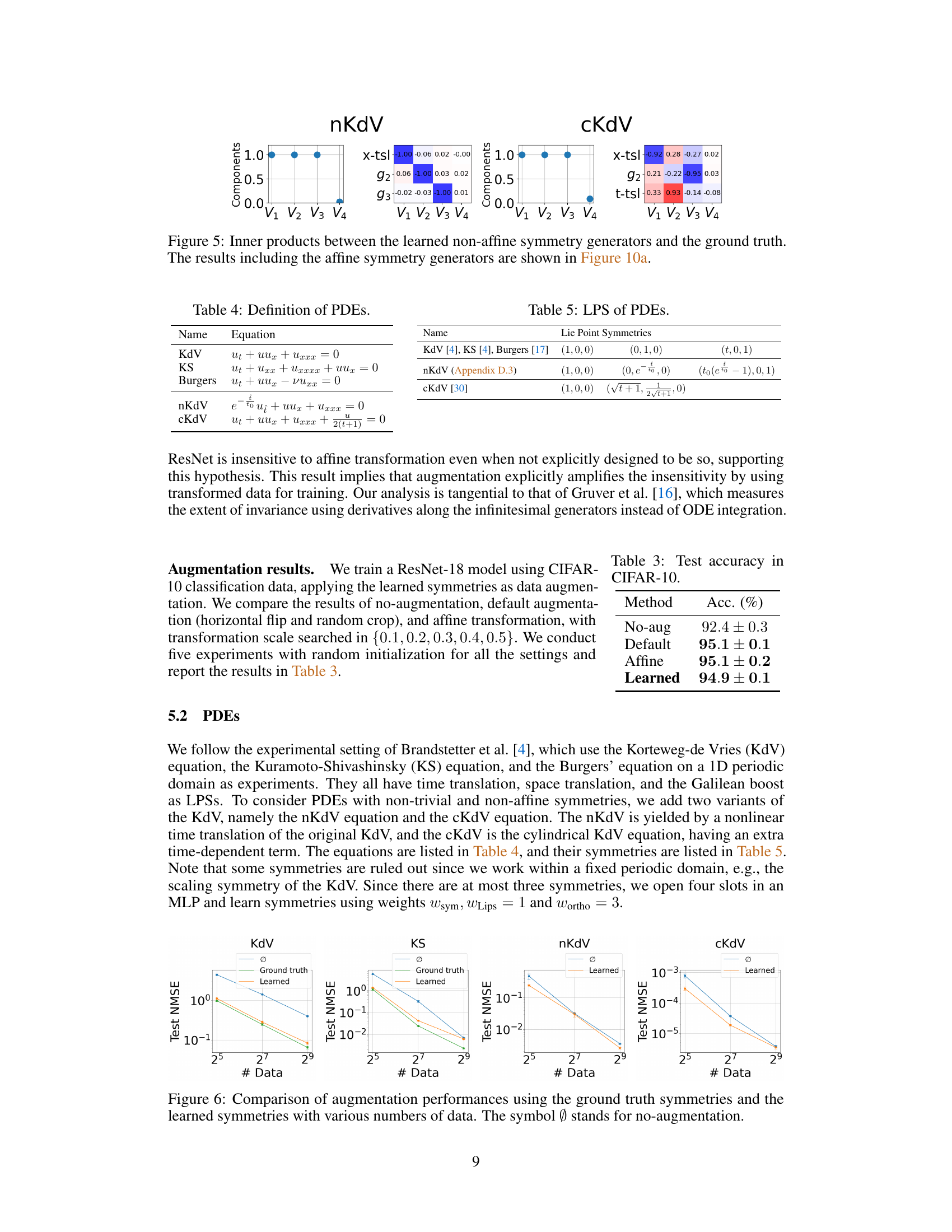
This figure compares the performance of data augmentation using ground truth symmetries and learned symmetries for four different partial differential equations (PDEs): KdV, KS, nKdV, and cKdV. The x-axis represents the number of data points used for training, and the y-axis represents the test normalized mean squared error (NMSE). The results show that augmentation with learned symmetries achieves comparable performance to augmentation with ground truth symmetries, especially when training data is scarce. The ‘Ø’ symbol indicates no augmentation.

This figure shows the weight function w(x) used in the Orthonormality loss. The weight function is designed to address the issue of varying importance of pixels in image datasets, where the center pixels often contain the main subject of the image and are more important than the boundary pixels. The weight function assigns higher weights to pixels closer to the center and lower weights to pixels further from the center. This ensures that the model focuses more on the central parts of images, which tend to be more informative. The figure displays a heatmap visualizing the weights, with brighter colors indicating higher weight.

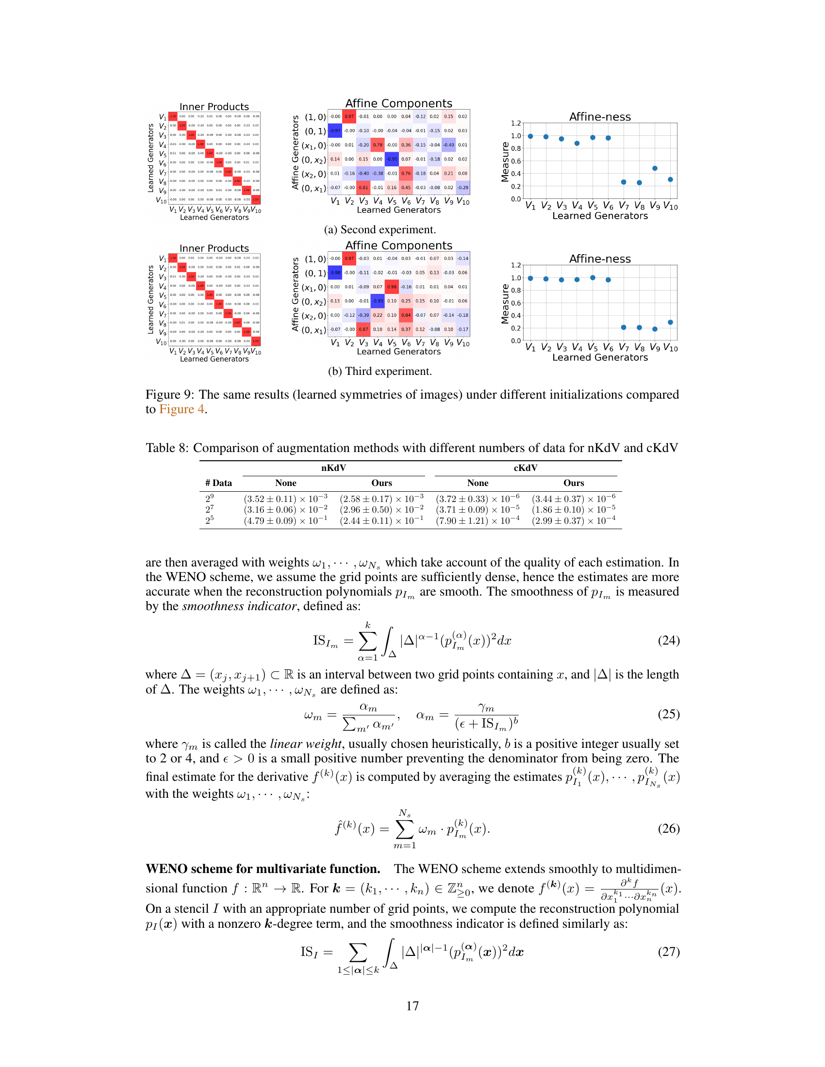
This figure shows the learned vector fields and their effect on the CIFAR-10 images. The left panel (a) visualizes the 10 learned vector fields, showing the direction and magnitude of the transformation at each pixel location. The right panel (b) displays the transformations of a sample image under different transformation scales, ranging from -0.3 to 0.3. The original, untransformed image corresponds to a transformation scale of 0.

This figure shows examples of learned vector fields, demonstrating the ability of the proposed method to identify symmetries in different domains. Panel (a) compares two vector fields, one representing a learned symmetry (V3, approximately rotation) and one not a symmetry (V7). Panel (b) illustrates transformed CIFAR-10 images using the learned generators, showcasing the effect of the learned symmetries on the image data. Panel (c) presents transformations of the Kuramoto-Sivashinsky (KS) equation, highlighting learned time translation and Galilean boost symmetries.
This figure shows examples of learned symmetries using the proposed method. (a) shows vector fields, where V3 represents a learned rotational symmetry while V7 is not a symmetry. (b) illustrates CIFAR-10 images transformed using the learned generators, highlighting the effect of the learned symmetries on the image data. (c) demonstrates transformations of the Kuramoto-Sivashinsky (KS) partial differential equation using learned symmetries, specifically time translation and Galilean boost. The figure visually demonstrates the method’s ability to identify and apply both approximate and exact symmetries.

This figure shows examples of learned symmetries from the proposed method. (a) shows vector fields learned from the CIFAR-10 dataset, where V3 is an approximately rotational symmetry and V7 is not a symmetry. (b) shows example transformed CIFAR-10 images using the learned generators. (c) shows the transformation of the Kuramoto-Sivashinsky (KS) equation with learned time translation and Galilean boost symmetries.
This figure shows examples of learned symmetries using the proposed method. (a) illustrates two vector fields, one representing a learned rotational symmetry (V3) and one that is not a symmetry (V7), highlighting the validity score’s ability to distinguish between them. (b) displays CIFAR-10 images transformed using the learned generators, showcasing the effects of the learned symmetries. (c) demonstrates the application of the method to partial differential equations (PDEs), specifically the Kuramoto-Sivashinsky (KS) equation, illustrating learned symmetries such as time translation and Galilean boost.

This figure visualizes the learned symmetries from the proposed method. (a) shows examples of vector fields learned, where V3 represents an approximate rotation symmetry, while V7 does not, resulting in a higher validity score. (b) demonstrates transformed CIFAR-10 images using these learned generators. (c) shows the application to PDEs, specifically the KS equation, illustrating the learned time translation and Galilean boost symmetries.

This figure shows examples of learned symmetries from the proposed method. (a) shows vector fields where V3 represents a learned rotation symmetry, while V7 is not a symmetry and has a high validity score. (b) visualizes transformed CIFAR-10 images using learned generators. (c) demonstrates the transformation of PDEs (KS equation) using learned time translation and Galilean boost symmetries.

This figure shows examples of learned symmetries on image and PDE data. Panel (a) displays vector fields learned by the model, with V3 approximating a rotation symmetry (low validity score) and V7 representing a non-symmetric transformation (high validity score). Panel (b) illustrates the CIFAR-10 images transformed using these learned generators, showcasing the effects of the learned symmetries. Panel (c) shows the transformation of the Kuramoto-Sivashinsky (KS) equation data using learned symmetries such as time translation and Galilean boost.

This figure shows examples of learned symmetries on image and PDE data. (a) shows vector fields learned by the model, where V3 represents a learned rotational symmetry while V7 does not. (b) shows CIFAR-10 images transformed using the learned generators. (c) shows the transformation of PDEs (KS equation) using learned symmetries such as time translation and Galilean boost.

This figure shows examples of learned symmetries using the proposed method. (a) shows vector fields, where V3 represents a learned rotational symmetry and V7 is not a symmetry. (b) presents transformed CIFAR-10 images using the learned generators, illustrating the effect of the learned symmetries on image data. (c) demonstrates the application of the method to partial differential equations (PDEs), specifically the Kuramoto-Sivashinsky (KS) equation, showcasing the learned time translation and Galilean boost symmetries.
More on tables
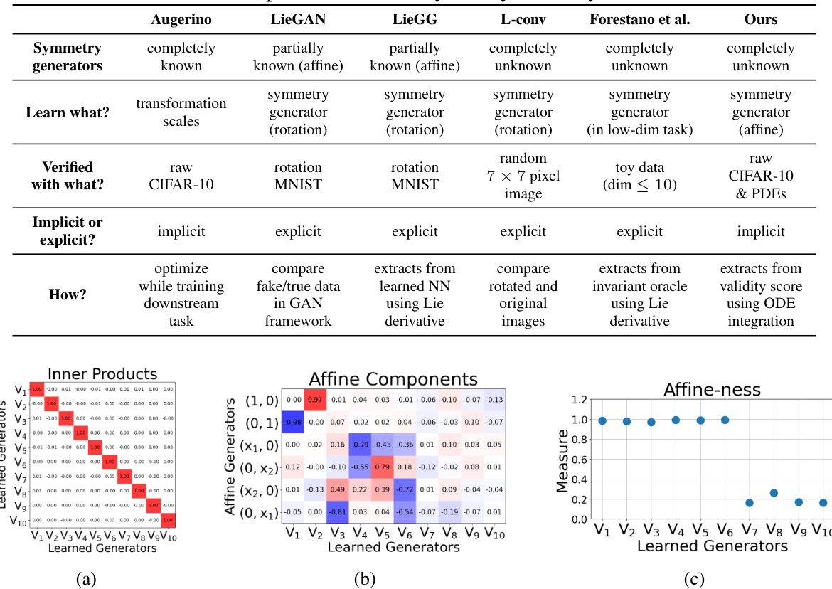
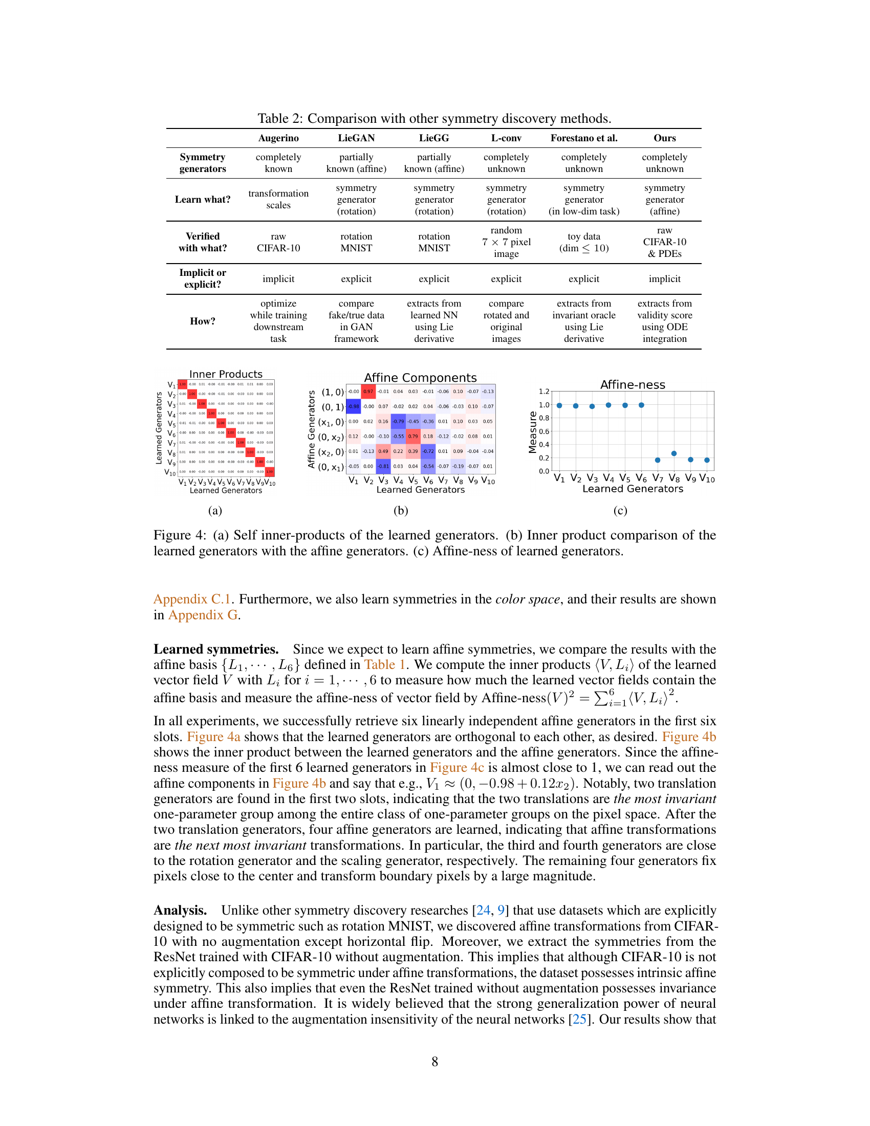
This table compares the proposed method with other state-of-the-art symmetry discovery methods. The comparison focuses on what is being learned (transformation scales vs. symmetry generators), the prior knowledge assumed (completely known, partially known, or unknown symmetry generators), whether the symmetry is implicit or explicit in the dataset, how the symmetry is learned, and whether the methods were tested on real-world or toy datasets. The table highlights the advantages of the proposed method in terms of its minimal assumptions and ability to work with high-dimensional real-world data.
This table compares the proposed method with other symmetry discovery methods, highlighting the differences in what is learned (transformation scales or subgroups), assumptions about prior knowledge (complete, partial, or none), and the viewpoint on symmetry (implicit or explicit). It emphasizes the proposed method’s advantages in handling high-dimensional real-world datasets and reducing the dimensionality of the search space.

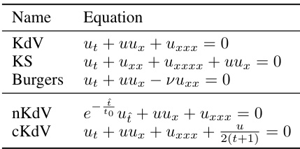
This table lists the Lie Point Symmetries (LPS) for several partial differential equations (PDEs): KdV, KS, Burgers, nKdV, and cKdV. For each PDE, the table shows the infinitesimal generators representing the symmetries. These symmetries describe transformations of the independent and dependent variables that leave the PDE invariant. The notation (ξ, μ) indicates the transformations on the independent variable x (ξ) and the dependent variable u (μ).
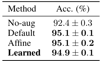
This table presents the test accuracy results (%) for image classification using CIFAR-10 dataset. Four different methods are compared: no augmentation, default augmentation (horizontal flip and random crop), augmentation using affine transformations, and augmentation using learned symmetries. The results show that both affine and learned symmetry augmentations significantly improve the accuracy compared to no augmentation and default augmentation.

This table presents the results of an experiment comparing different data augmentation methods for training Fourier Neural Operators (FNOs) on the cylindrical Korteweg-de Vries (cKdV) equation. The methods compared are no augmentation, augmentation using Lie Point Symmetries (LPS), augmentation using Approximate Symmetries (AS), and augmentation using both LPS and AS. The table shows the Normalized Mean Squared Error (NMSE) for two different dataset sizes (25 and 27 data points). Lower NMSE indicates better performance.

This table compares the performance of three different augmentation methods (None, Ground-truth, and Ours) on two partial differential equations (KdV and KS) with varying amounts of training data (25, 27, and 29 data points). The ‘None’ column represents no augmentation. ‘Ground-truth’ utilizes augmentations based on known symmetries. The ‘Ours’ column uses augmentations generated by the proposed method. The results show the NMSE (Normalized Mean Squared Error) for each method and dataset size, demonstrating how the proposed method compares to using known symmetries and no augmentation at all.

This table compares the performance of different data augmentation methods on two variations of the Korteweg-de Vries equation (nKdV and cKdV). The ‘None’ column represents no augmentation, while the ‘Ours’ column shows the results when using the learned symmetries from the proposed method. The Normalized Mean Squared Error (NMSE) is reported for various dataset sizes (25, 27, 29 data points). Lower NMSE values indicate better model performance.

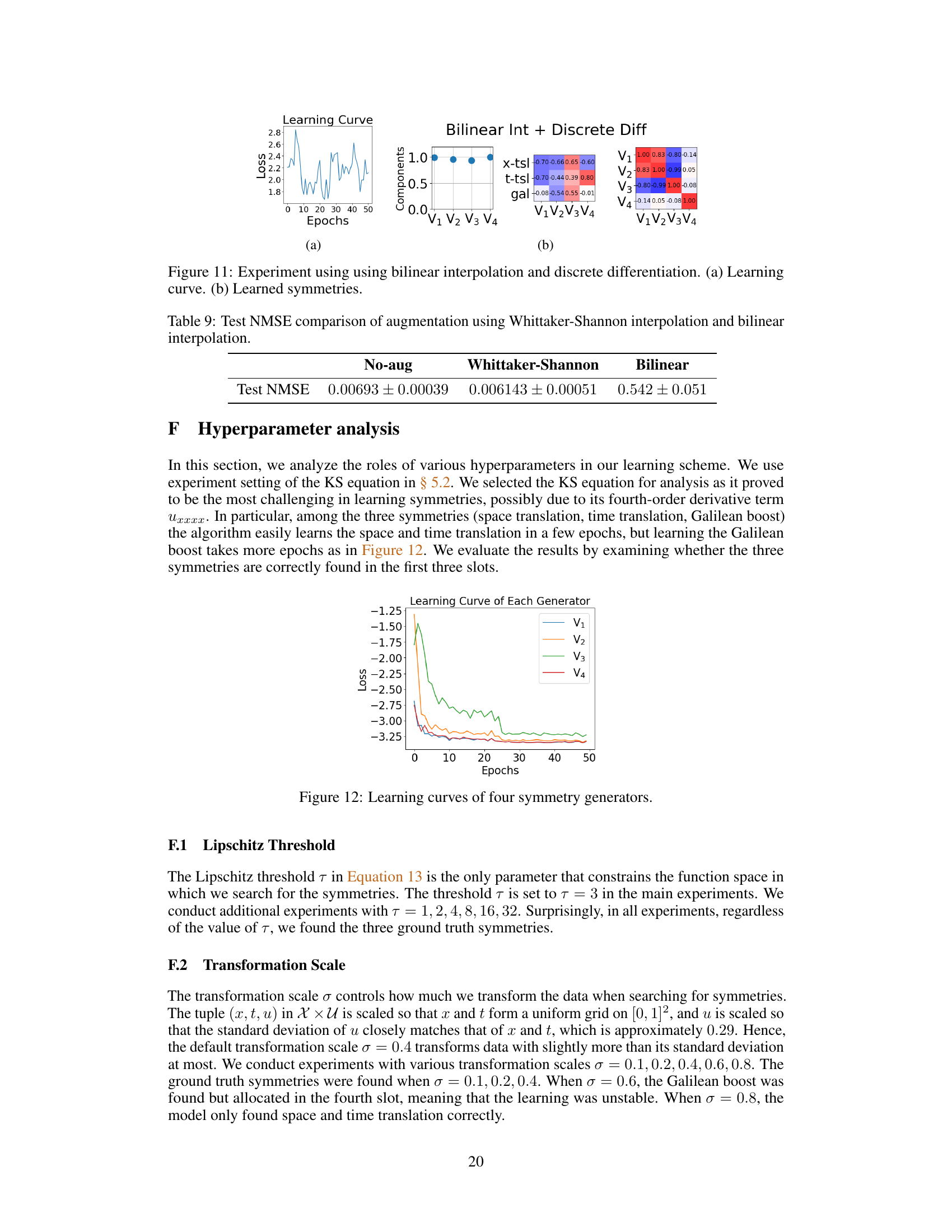
This table presents a comparison of the test Normalized Mean Squared Error (NMSE) for the Kuramoto-Sivashinsky (KS) equation using three different augmentation methods: No augmentation, Whittaker-Shannon interpolation, and bilinear interpolation. The results show a significant improvement in NMSE when using Whittaker-Shannon interpolation compared to the other two methods.

This table presents the results of a hyperparameter study on the weights of the three loss functions (symmetry loss, orthonormality loss, Lipschitz loss) used in the symmetry learning algorithm. It shows how many of the three expected symmetries were correctly learned in the first three slots of the model for various combinations of the weights. This helps determine appropriate weighting of the losses for optimal symmetry discovery.
Full paper#


