↗ OpenReview ↗ NeurIPS Homepage ↗ Chat
TL;DR#
Analyzing turbulent fluid flow is crucial but computationally challenging. 3D Particle Tracking Velocimetry (PTV) is a key technique, relying heavily on dual-frame fluid motion estimation algorithms. Traditional methods are limited by the need for large, labeled datasets. Existing deep learning approaches, while improving accuracy, still rely on supervised learning and thus suffer from the same data limitations. This reliance on large labeled datasets is costly and time-consuming to acquire, making it difficult to analyze specialized scenarios or less-common flow types.
This research introduces FluidMotionNet, a novel self-supervised method for dual-frame fluid motion estimation. The core innovation is a zero-divergence loss function, efficiently implemented using a splat-based approach, which is tailored to the specific characteristics of fluid flow. This self-supervised nature enables test-time optimization, leading to a dynamic velocimetry enhancer module that further improves accuracy. The results show that FluidMotionNet significantly outperforms existing supervised methods, even with a mere 1% of their training data. This demonstrates remarkable data efficiency and cross-domain robustness.
Key Takeaways#
Why does it matter?#
This paper is significant because it presents a self-supervised method for 3D fluid motion estimation that surpasses supervised methods while using only 1% of the training data. This significantly reduces data collection needs and improves cross-domain robustness, opening new avenues for analyzing turbulent flow in various applications. Its efficient test-time optimization further enhances its practical value.
Visual Insights#

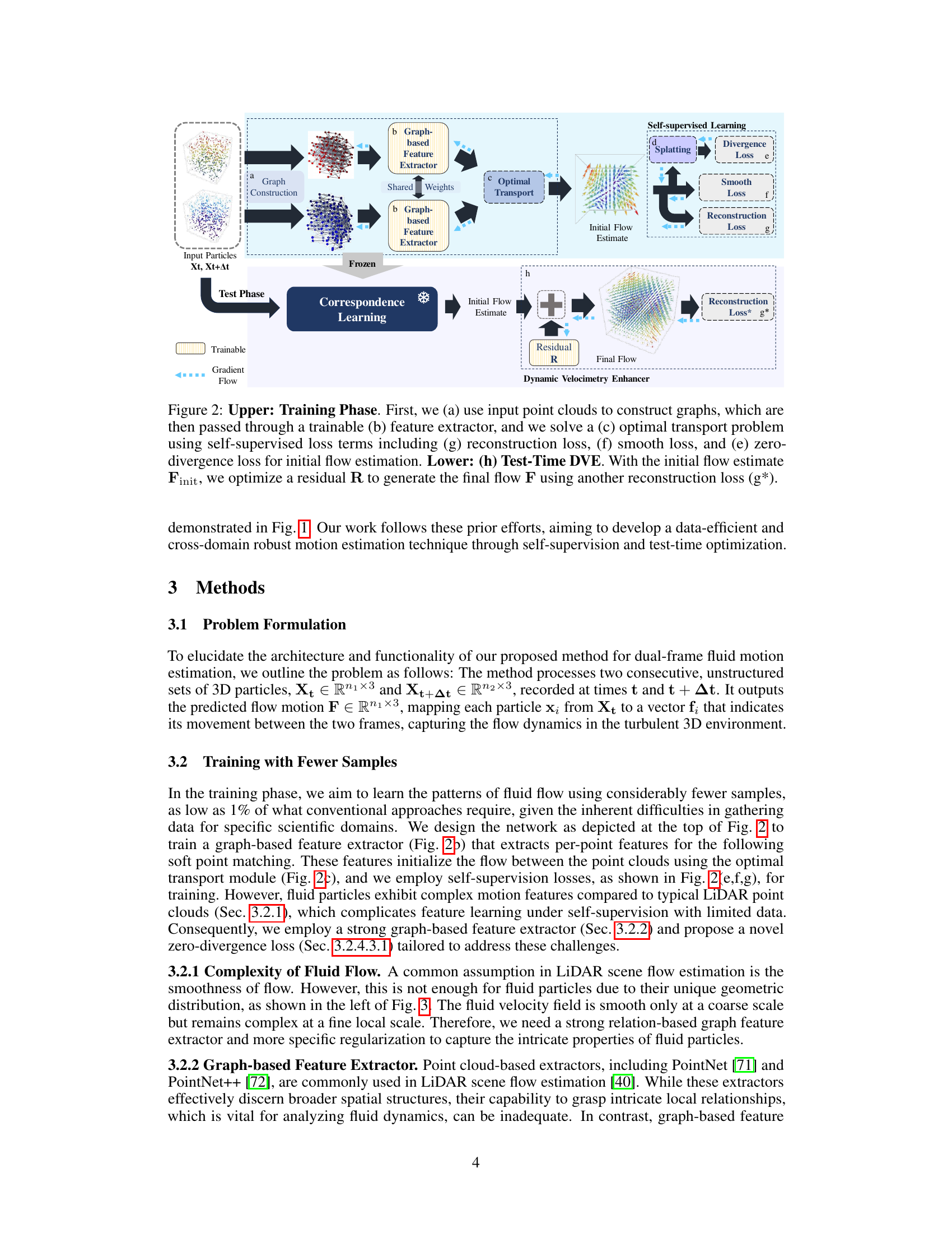
This figure compares three different approaches for dual-frame fluid motion estimation: DeepPTV, GotFlow3D, and the proposed method. It highlights the shift from supervised, iterative methods (DeepPTV) to supervised methods using correspondence and residual learning (GotFlow3D) and finally to a self-supervised method leveraging a Dynamic Velocimetry Enhancer (DVE) for test-time optimization. The self-supervised nature allows for superior performance with less training data. The snowflake icon represents frozen weights during test time.
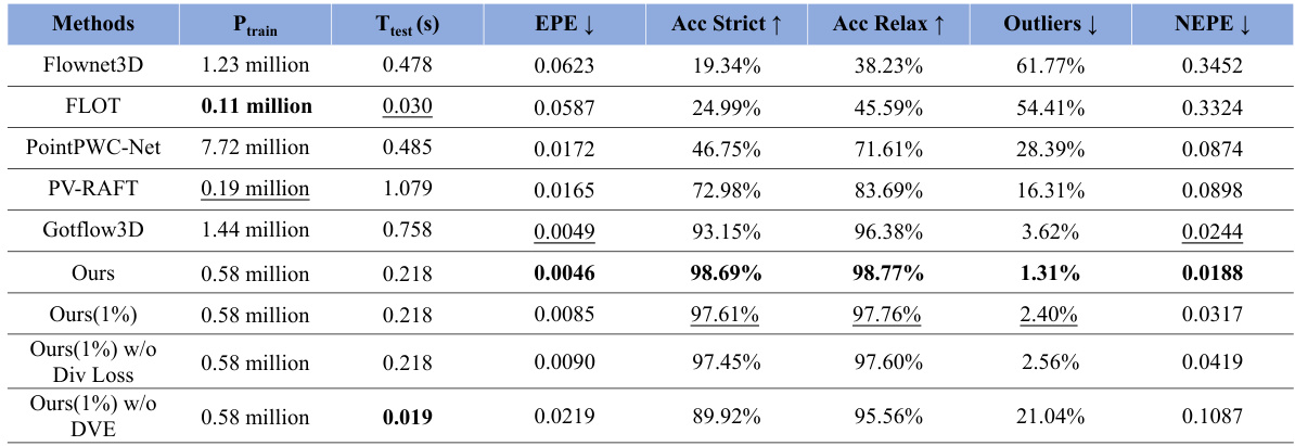
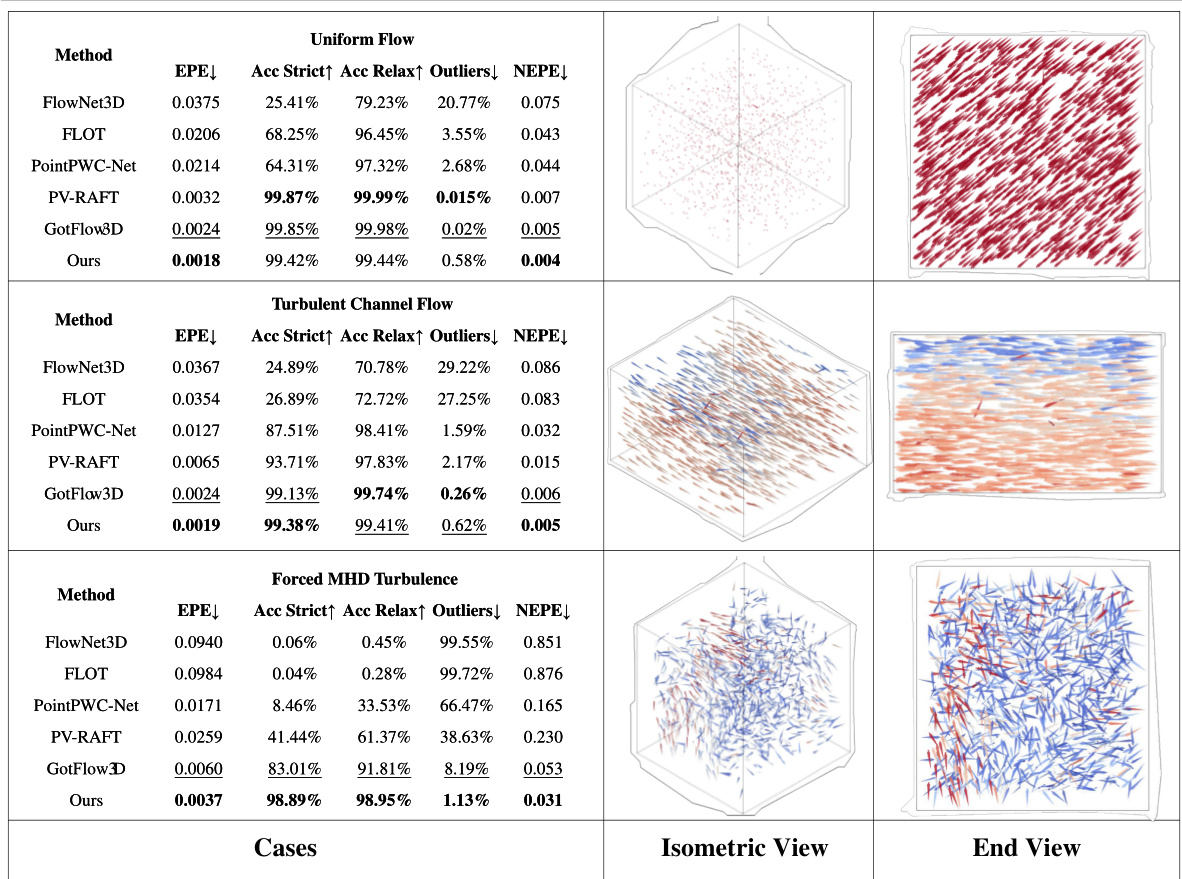
This table compares the proposed self-supervised method against several fully supervised state-of-the-art methods for dual-frame fluid motion estimation. The top part shows the number of parameters, inference time, and various metrics (EPE, accuracy, outliers, NEPE) when all models are trained on the full dataset. The bottom part shows a breakdown of the performance across three representative flow cases (Uniform Flow, Turbulent Channel Flow, Forced MHD Turbulence) from the FluidFlow3D dataset, again comparing the proposed method to the fully supervised methods. The table highlights the superior performance of the proposed method, particularly when trained on only 1% of the data.
In-depth insights#
Self-Supervised PTV#
Self-supervised PTV presents a compelling paradigm shift in 3D particle tracking velocimetry. Traditional PTV methods heavily rely on labeled data for training, a process that’s often expensive and time-consuming. Self-supervised approaches, however, leverage the inherent structure and properties of fluid flow to learn from unlabeled data, significantly reducing the need for manual annotation. This is achieved through innovative loss functions that enforce physical constraints such as zero-divergence in incompressible fluid flows. By incorporating such domain-specific knowledge directly into the learning process, self-supervised PTV demonstrates superior performance while maintaining data efficiency. Furthermore, the self-supervised nature allows for test-time optimization, dynamically adapting the model to unseen data and scenarios, thereby enhancing robustness and generalization capabilities. This approach promises to overcome major limitations in 3D PTV, particularly concerning the acquisition of large, fully annotated datasets, and opens avenues for broader application in areas where labeled data is scarce or impractical to obtain.
Zero-Divergence Loss#
The concept of “Zero-Divergence Loss” in the context of fluid motion estimation is a significant contribution, addressing the inherent physical constraint of incompressible fluid flow. This loss function directly enforces the zero-divergence property, ensuring that the estimated velocity field accurately reflects the behavior of incompressible fluids. The authors cleverly implement this loss using a splatting technique, effectively mapping the sparse, irregular particle data onto a regular grid for efficient computation. This approach enables the training of a model that learns the complex dynamics of fluid flows with better fidelity. The effectiveness of zero-divergence loss is particularly crucial in situations where data is limited, as it provides a strong inductive bias guiding the model’s learning, leading to improved accuracy even with a smaller training set. The authors demonstrate the advantage of their approach through superior cross-domain robustness and performance gains compared to state-of-the-art methods which rely on fully supervised learning.** The integration of zero-divergence loss represents a compelling advancement in self-supervised learning for fluid mechanics.**
Test-Time Optimization#
Test-time optimization (TTO) is a crucial technique to enhance the performance of deep learning models, particularly in scenarios with limited training data or significant domain shift. TTO refines a pre-trained model’s parameters during the testing phase, adapting it to unseen data or specific characteristics of the input without requiring additional training labels. This addresses the limitations of traditional supervised learning, where large annotated datasets are often necessary for optimal results. The key advantage of TTO is its ability to leverage the inherent structure and information within the test data itself for model adaptation, making it especially valuable in applications with data scarcity or significant domain differences. A further benefit is the improved efficiency as TTO avoids retraining the whole model, leading to reduced computation time and cost. While TTO offers significant advantages, it’s important to address potential risks, such as overfitting to individual test samples and maintaining the model’s generalization capabilities to unseen future data. Proper regularization and careful consideration of the optimization strategy are critical to ensure TTO’s effectiveness and robustness.
Cross-Domain Robustness#
Cross-domain robustness in this research paper refers to a model’s ability to generalize its performance to unseen domains. The authors address the challenge of limited data in specific scientific domains, where collecting diverse and representative Particle Tracking Velocimetry (PTV) datasets is inherently difficult. Their proposed self-supervised framework, including a novel zero-divergence loss and Dynamic Velocimetry Enhancer (DVE) module, is shown to be remarkably robust across various synthetic and real-world domains. This robustness is demonstrated through experiments involving leave-one-out cross-validation on synthetic datasets and evaluations on real physical and biological datasets. The test-time optimization capabilities of the method are highlighted, where the DVE module adapts the model’s performance to unseen domains in a way that improves data efficiency and generalizability. The results underscore the practical value of the approach for real-world 3D PTV applications, where data scarcity and domain shift are frequent challenges.
Limited Data Learning#
Limited data scenarios pose a significant challenge in training effective machine learning models, especially in specialized domains like fluid dynamics where data acquisition is often complex and expensive. This paper tackles this challenge by introducing a novel self-supervised approach for dual-frame fluid motion estimation. The self-supervised nature eliminates the need for large labeled datasets, a major advantage over existing supervised methods. This approach employs a new zero-divergence loss, specific to fluid dynamics, and a splat-based implementation for efficient computation. Furthermore, the self-supervised framework inherently supports test-time optimization, resulting in a robust and cross-domain adaptable model, even with limited training samples. The authors demonstrate superior performance compared to supervised counterparts, achieving state-of-the-art results with only 1% of the training data used by supervised models. The model’s robustness and data efficiency make it highly promising for various applications where large labeled datasets are unavailable.
More visual insights#
More on figures

This figure compares three different approaches for dual-frame fluid motion estimation: DeepPTV, GotFlow3D, and the proposed method. DeepPTV and GotFlow3D are supervised methods using labeled data for training. The proposed method is self-supervised and leverages a Dynamic Velocimetry Enhancer (DVE) module for test-time optimization, allowing it to adapt to unseen data during testing. The figure highlights the key differences in architecture and training paradigms between these methods.

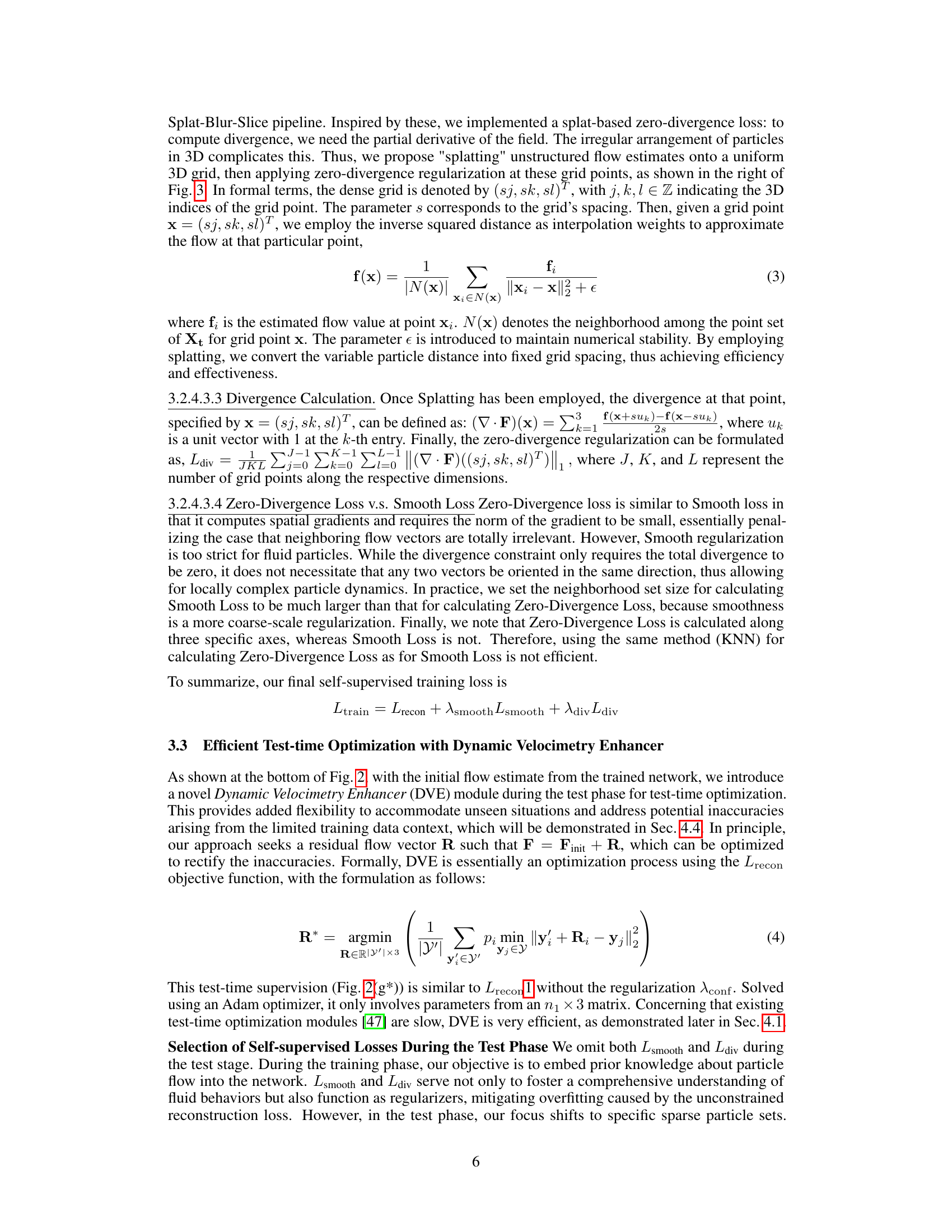
The figure visualizes the process of calculating the zero-divergence loss used in the training phase. The left panel shows a sample of the FluidFlow3D dataset, illustrating the complex, non-uniform nature of turbulent fluid flows. The right panel details the splatting-based method for computing the divergence loss. The sparse flow field (from the initial flow estimate) is ‘splatted’ or interpolated onto a regular 3D grid. This process enables the calculation of the divergence at each grid point, allowing for efficient minimization of the zero-divergence loss that is critical to representing the incompressible nature of fluids.
This figure illustrates the difference between existing supervised dual-frame fluid motion estimation methods (DeepPTV and GotFlow3D) and the proposed self-supervised method. It highlights the key difference being the use of test-time optimization in the proposed method to improve accuracy and robustness, while also showing the reduction in the required training data.

This figure compares the proposed self-supervised method against fully supervised state-of-the-art methods on the FluidFlow3D dataset. The top part shows a comparison of the trainable parameters count, inference time per sample, and various performance metrics. The bottom part presents the performance across six different flow cases, with visualizations provided for three representative cases.

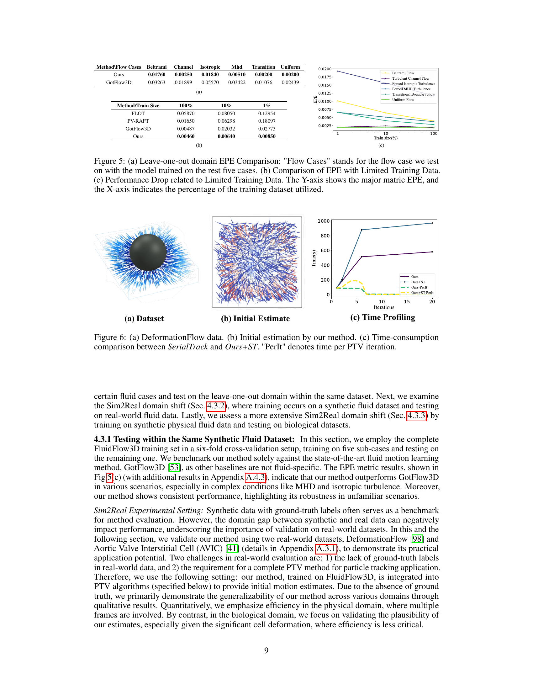
This figure shows three subplots that illustrate different aspects of the proposed method’s performance, especially in the context of real-world data. Subplot (a) displays the DeformationFlow dataset, highlighting the unique characteristics of real-world fluid flow data. Subplot (b) presents the initial flow estimation results produced by the proposed method, demonstrating its ability to estimate fluid motion from unstructured data. Lastly, subplot (c) provides a detailed comparison of the time consumption between the proposed method and the SerialTrack method, across various iterations, showing the efficiency gains achieved by incorporating the proposed method’s initial estimation into the workflow.
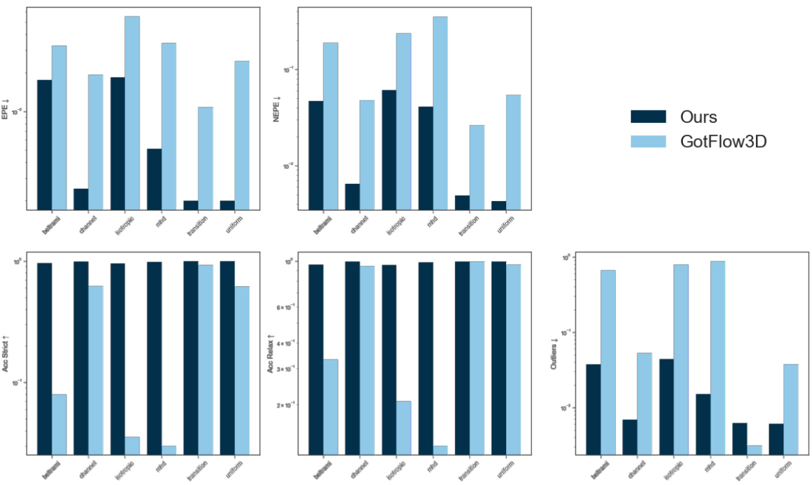
This figure presents a comparison of the proposed self-supervised method against several fully supervised state-of-the-art methods for dual-frame fluid motion estimation. The top part shows a quantitative comparison in terms of trainable parameters, inference time, End Point Error (EPE), accuracy (strict and relaxed), and outlier rates. The bottom part shows the performance across six different flow cases from the FluidFlow3D dataset, highlighting the superior performance of the proposed method, particularly in complex flow scenarios.
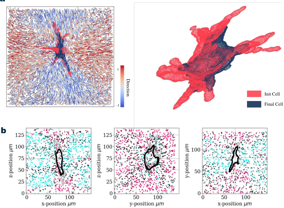
This figure visualizes the results of the proposed method on the Aortic Valve Interstitial Cell (AVIC) dataset. Panel (a) shows a 3D rendering of a cell, highlighting the deformation before and after treatment with Cytochalasin-D, a drug that affects cell structure. Panel (b) provides 2D projections of the flow field along the x, y, and z axes, showing the direction and magnitude of movement of particles near the cell. The visualizations help demonstrate the method’s ability to capture detailed movement in complex biological scenarios.

This figure shows the convergence of the End Point Error (EPE) metric during the test-time optimization process using the Dynamic Velocimetry Enhancer (DVE) module. The x-axis represents the number of iterations in the optimization process, and the y-axis shows the EPE value. The graph demonstrates that the EPE decreases rapidly in the initial iterations and then gradually converges to a stable, low error value after around 150-200 iterations. This illustrates the efficiency of the DVE module in refining the initial flow estimation within a relatively small number of optimization steps.
More on tables

This table presents a comparison of the performance of two methods, Fm-track and Ours+Fm, on the AVIC dataset. Three different experimental settings (C2E, C2N, E2N) representing different treatment combinations are used. The table shows the number of tracked matches and the mean neighbor distance score (MNDS). A lower MNDS indicates better accuracy.

This table compares the performance of four different methods (FLOT, PV-RAFT, Gotflow3D, and the proposed ‘Ours’ method) for 3D fluid motion estimation under varying training data sizes (100%, 10%, and 1%). The metrics used are End-Point Error (EPE), Accuracy Strict, Accuracy Relaxed, and Outliers. The results show the robustness of the proposed method to limited data, maintaining high accuracy with low outlier rates even when trained on only 1% of the data.

This table compares the performance of four different methods (FLOT, PV-RAFT, Gotflow3D, and the proposed ‘Ours’ method) for 3D fluid motion estimation under varying training data sizes (100%, 10%, and 1%). The metrics used to evaluate performance are End-Point Error (EPE), Accuracy Strict, Accuracy Relaxed, and the percentage of Outliers. The results demonstrate the robustness of the ‘Ours’ method, which maintains high accuracy and low outlier rates even with significantly reduced training data.
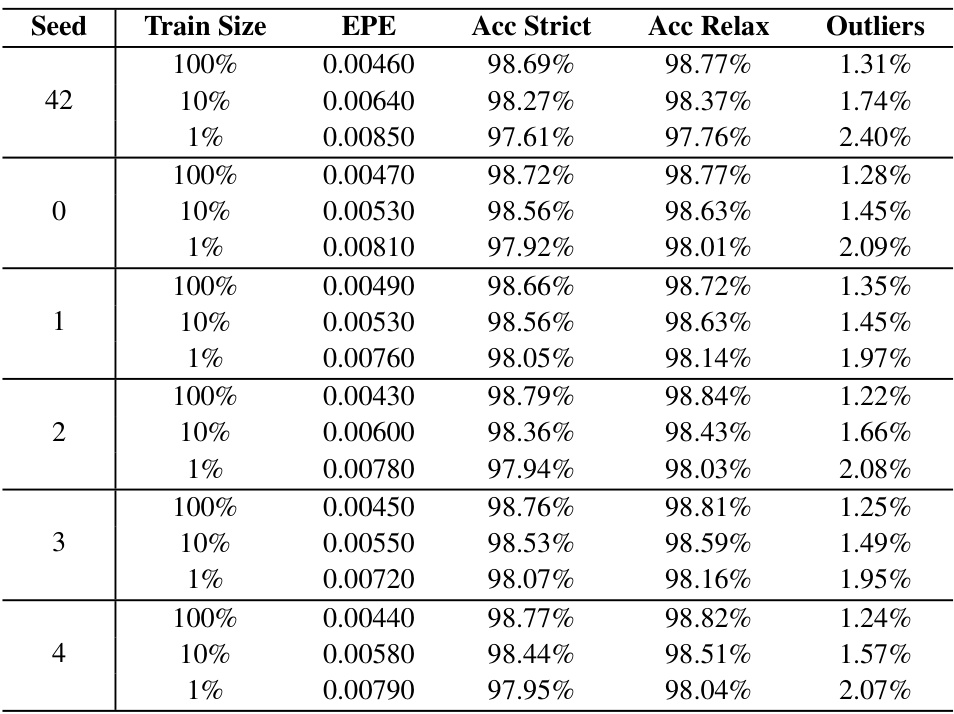
This table compares the performance of four different methods (FLOT, PV-RAFT, GotFlow3D, and the proposed method) for 3D fluid motion estimation using varying amounts of training data (100%, 10%, and 1%). The metrics used are End-Point Error (EPE), Accuracy Strict, Accuracy Relaxed, and Outliers. The results show that the proposed method is robust to reductions in training data size, maintaining high accuracy and low outlier rates.

This table compares the performance of the proposed graph-based feature extractor against PointNet++, a commonly used point cloud feature extractor. Both models were trained using the full FluidFlow3D dataset. The comparison uses EPE, Acc Strict, Acc Relax, and Outliers metrics to evaluate performance.

This table compares the performance of the proposed method with and without the zero-divergence loss term on the FluidFlow3D test dataset. The results are presented for three different training data sizes (100%, 10%, and 1%). The metrics used are End Point Error (EPE), Accuracy Strict, Accuracy Relaxed, and Outliers. Bold values indicate better performance compared to the model without the zero-divergence loss.
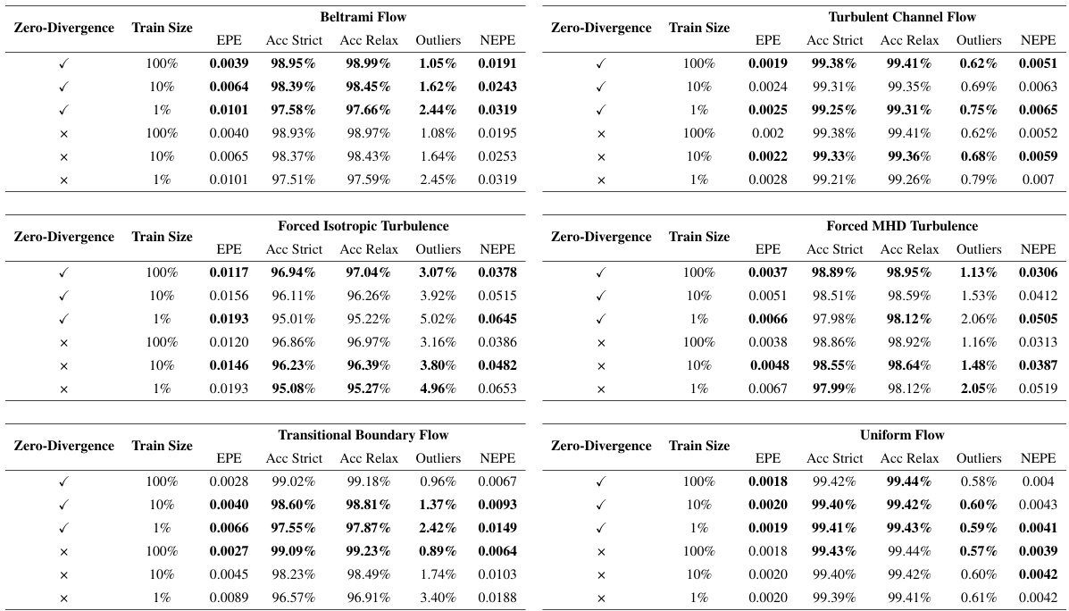
This table compares the performance of four different methods (FLOT, PV-RAFT, Gotflow3D, and the proposed ‘Ours’ method) on a fluid flow estimation task using varying amounts of training data (100%, 10%, and 1%). The results, measured by End-Point Error (EPE), Accuracy Strict, Accuracy Relaxed, and Outliers, demonstrate the robustness of the ‘Ours’ method, showing its ability to maintain high accuracy and low outlier rates even with significantly less training data.

This table presents a comparison of the model’s performance with and without the Dynamic Velocimetry Enhancer (DVE) module, across different training data sizes (100%, 10%, and 1%). The metrics used for evaluation include End-Point Error (EPE), Accuracy Strict, Accuracy Relax, and Outliers. The results show that the DVE module significantly improves performance, particularly with smaller training datasets.
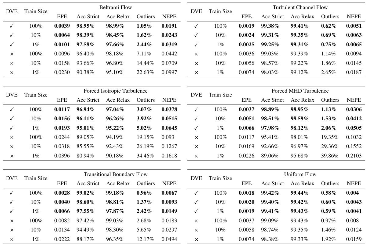
This table compares the performance of four different methods (FLOT, PV-RAFT, Gotflow3D, and Ours) for estimating fluid motion using varying amounts of training data (100%, 10%, and 1%). The results show the end-point error (EPE), accuracy (strict and relaxed), and outlier percentages for each method and training data size. The key finding is that the ‘Ours’ method is more robust to reduced training data, maintaining high accuracy and low outlier rates.

This table compares the performance of four different methods (FLOT, PV-RAFT, Gotflow3D, and Ours) for 3D fluid motion estimation using different amounts of training data (100%, 10%, and 1%). The metrics used for comparison are End-Point Error (EPE), Accuracy Strict, Accuracy Relaxed, and Outliers. The results demonstrate the robustness of the ‘Ours’ method, which maintains high accuracy and low outlier rates even with significantly reduced training data.
Full paper#
