The Feature Speed Formula: a flexible approach to scale hyper-parameters of deep neural networks

↗ OpenReview ↗ NeurIPS Homepage ↗ Chat

TL;DR

#

Key Takeaways

#

Why does it matter?

#

This paper is crucial for researchers working on deep learning optimization because it provides a novel theoretical framework for understanding and controlling the feature learning process in deep neural networks. It offers practical guidance for hyperparameter tuning, improving training efficiency and performance. This work opens avenues for developing novel architectures and optimization algorithms tailored for specific learning behaviors.

Visual Insights

#

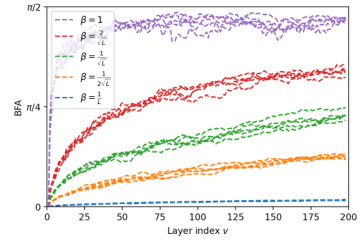
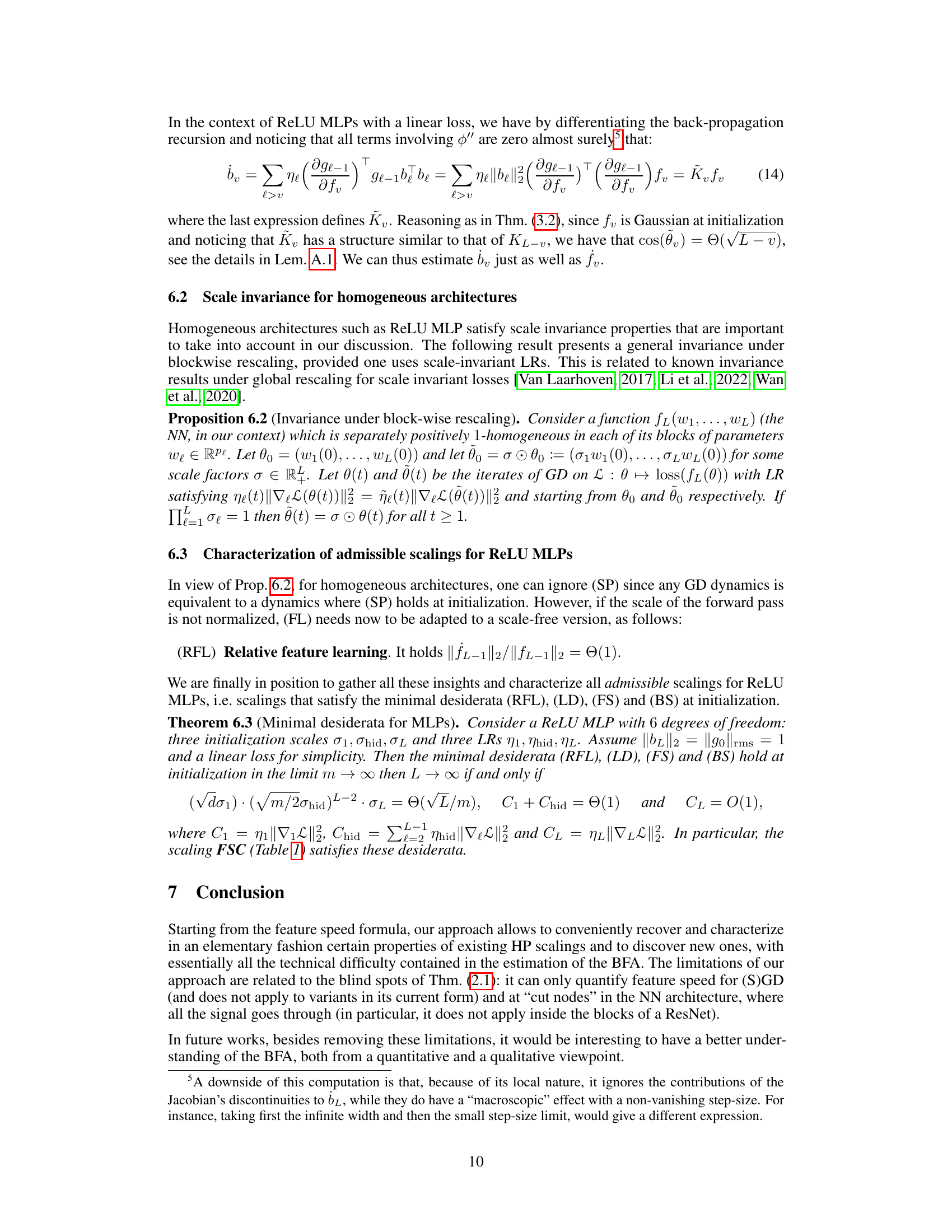
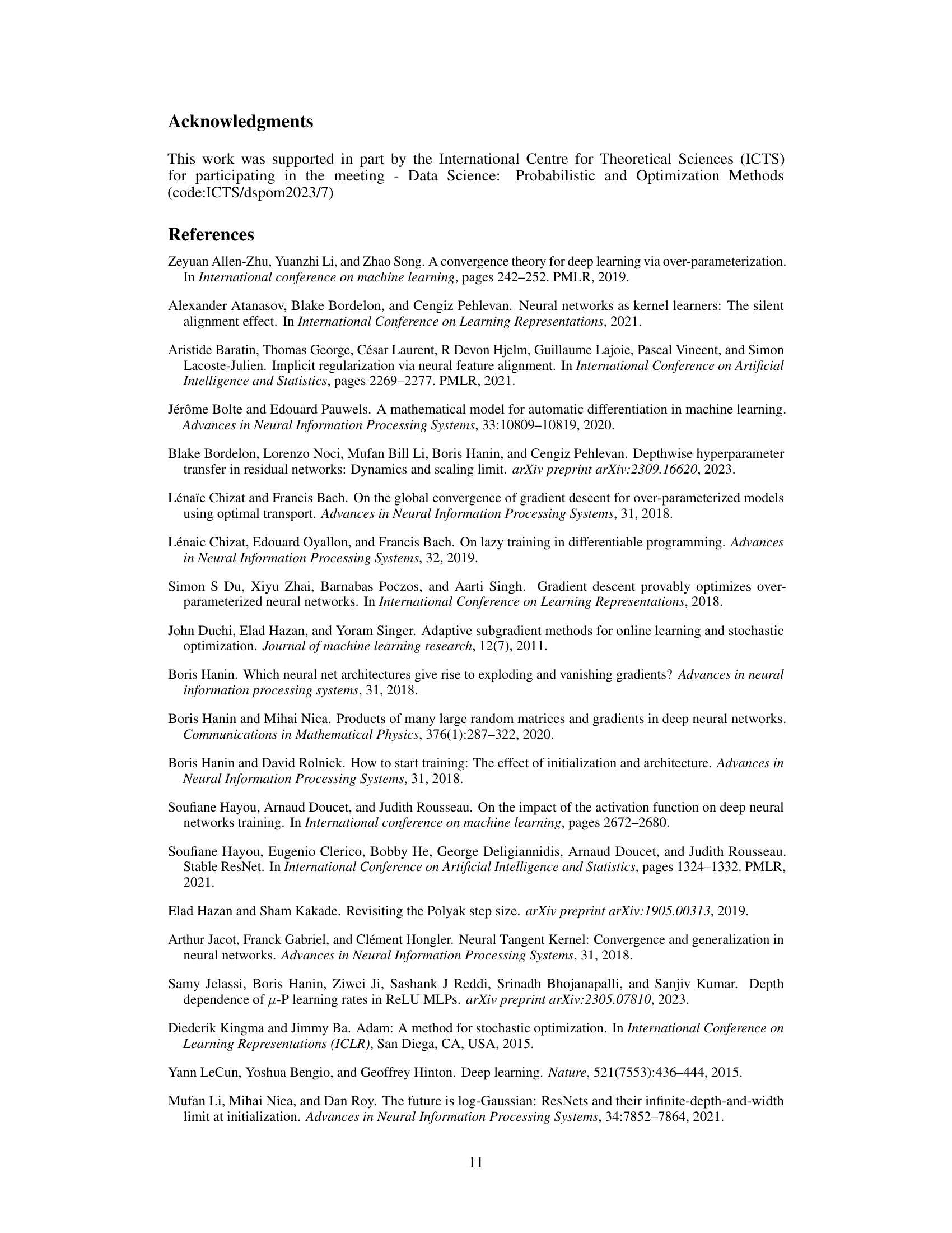
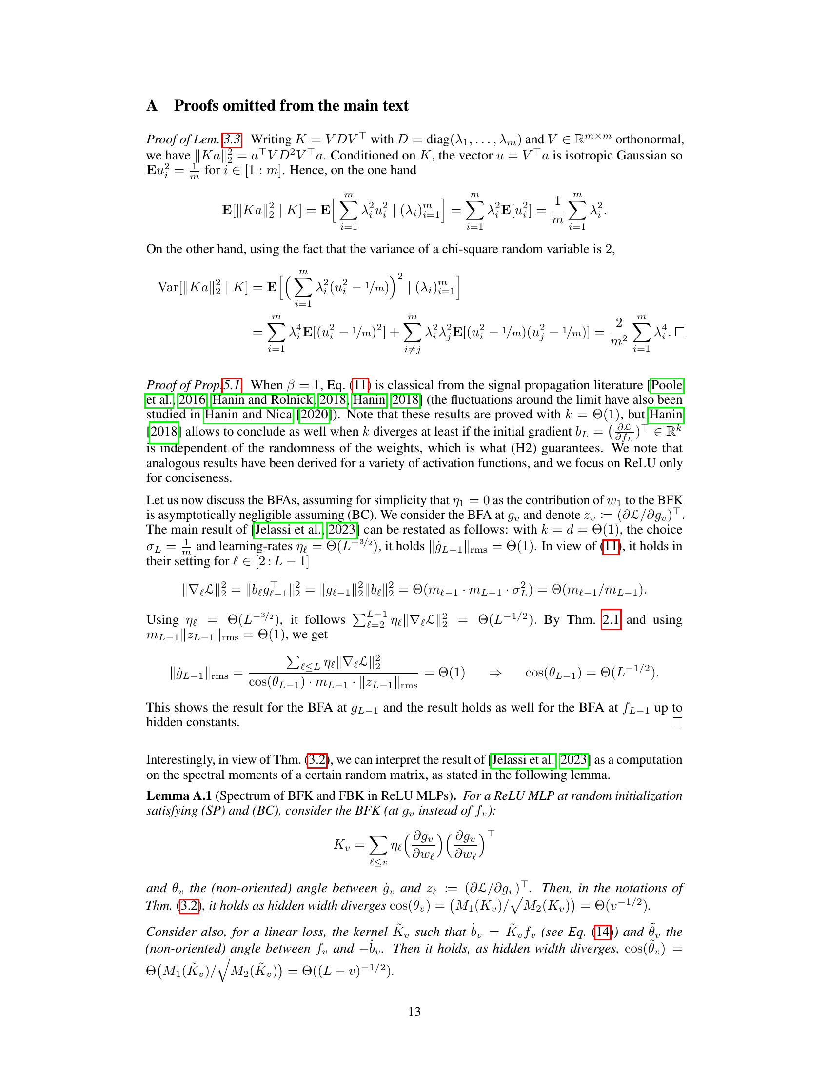
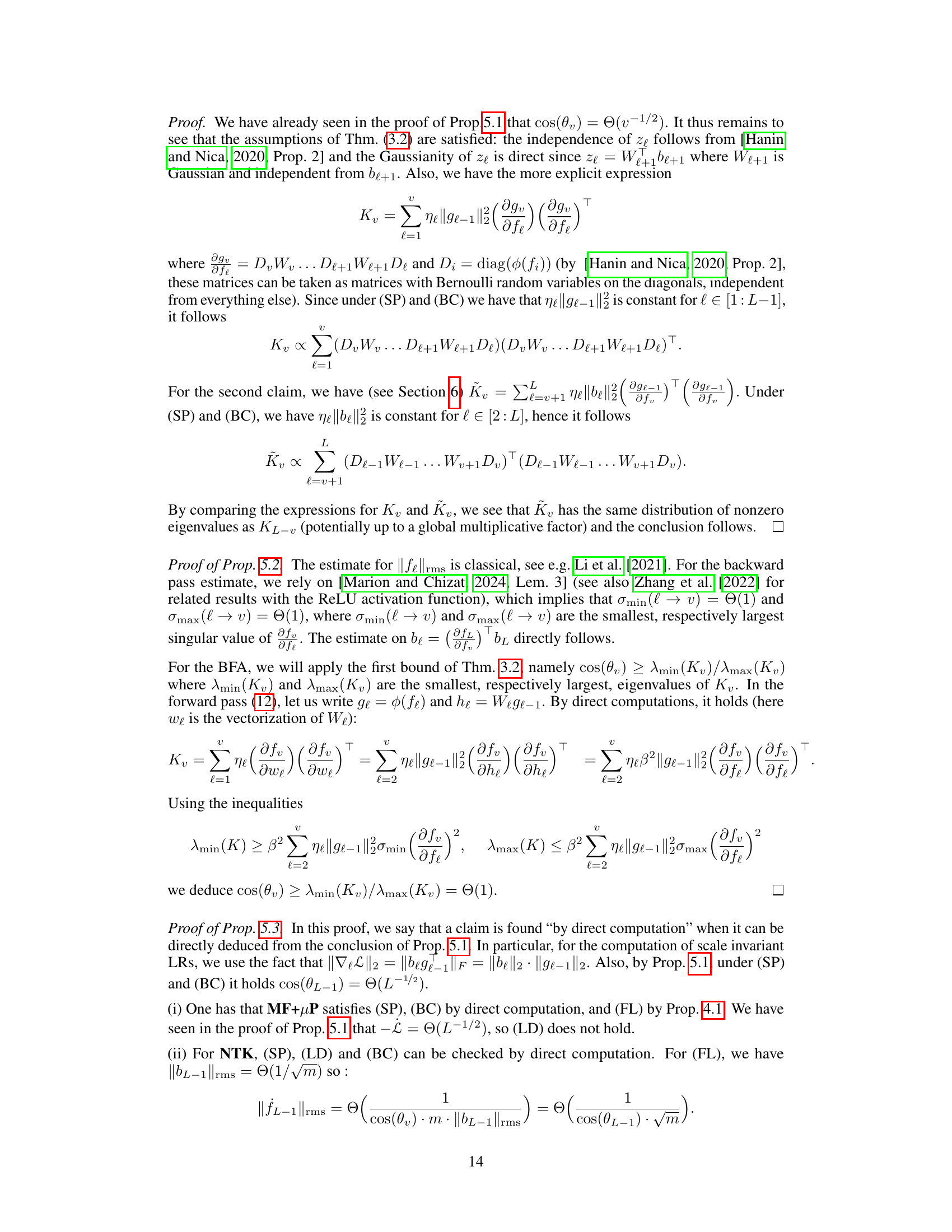
This figure shows the Backward-Feature Angle (BFA) at initialization for MLPs and ResNets with varying architectures. Panel (a) demonstrates that the BFA changes in the initial layers before stabilizing. Panel (b) shows that the BFA at the output layer is asymptotically independent of depth, but only when the branch scale is proportional to 1/√L. Lastly, panel (c) illustrates that the asymptotic output BFA is directly determined by the branch scale.

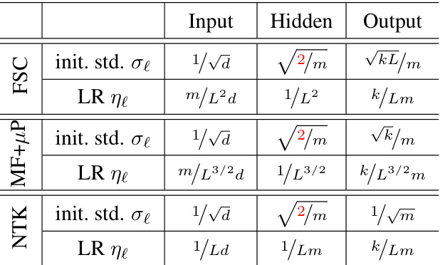
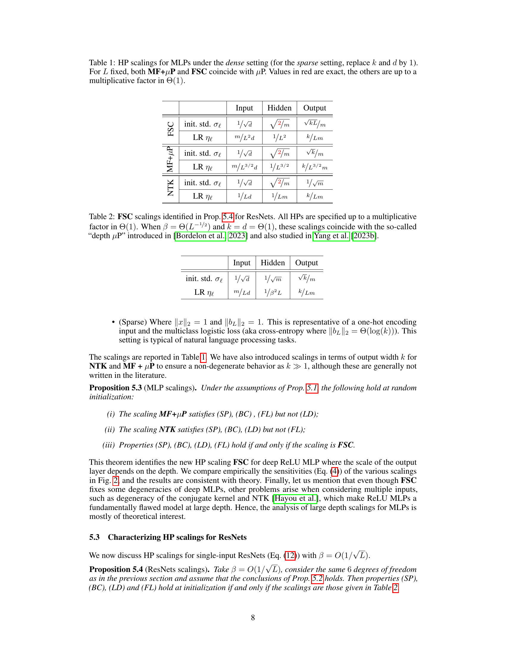
This table presents a comparison of three different hyperparameter (HP) scaling schemes for Multilayer Perceptrons (MLPs) under two settings: dense and sparse. For each scaling (NTK, MF+µP, FSC), it shows the initialization standard deviation (init. std. σℓ) and learning rate (LR ηℓ) for the input, hidden, and output layers. The ‘dense’ setting represents a scenario with a dense input and a dense output, while the ‘sparse’ setting would involve sparse inputs and outputs. The table highlights that for a fixed depth (L), the MF+µP and FSC scalings are equivalent to the µP scaling.

In-depth insights

#

Feature Speed Formula

#

The conceptualization of a ‘Feature Speed Formula’ in a deep learning context is intriguing. It suggests a mechanism to quantify and predict the rate of feature learning during training, a notoriously opaque process. The core idea seems to be establishing a relationship between the speed of feature updates, the angle between feature updates and backward passes, and loss decay. This formula, if valid, would provide a powerful tool to understand and potentially optimize hyperparameters. For instance, by analyzing the angle between feature updates and the backward pass, one might gain insight into how different initializations and learning rate schedules influence learning dynamics. A practical application might involve adjusting hyperparameters to achieve desirable properties (e.g., feature learning speed, loss decay) by targeting specific values for the aforementioned angle. The success of such an approach hinges on the formula’s generalizability across diverse network architectures and the ability to accurately estimate the key angle in practice. Further research should explore these aspects to validate the formula’s practical applicability and broader implications for deep learning research.

BFK Spectrum Analysis

#

A hypothetical ‘BFK Spectrum Analysis’ section in a deep learning research paper would likely explore the spectral properties of the Backward-to-Feature Kernel (BFK). The BFK maps backward pass vectors to feature updates, providing a crucial link between gradient information and feature learning dynamics. Analyzing the BFK’s spectrum could reveal critical insights into training stability and generalization. For instance, a well-conditioned BFK (eigenvalues clustered around 1) might suggest efficient signal propagation and effective feature learning, leading to faster convergence and better generalization. Conversely, a poorly conditioned BFK could indicate difficulties in training, such as vanishing or exploding gradients. The analysis might also delve into the relationship between the BFK spectrum and hyperparameter choices. Optimal hyperparameter settings might be linked to specific spectral properties, ensuring a well-behaved BFK across layers and contributing to enhanced performance. The study could employ both theoretical analyses and empirical investigations, potentially comparing results across various network architectures and training regimes. Understanding how the BFK spectrum evolves during training is equally important, allowing researchers to track changes in feature learning dynamics and diagnose potential training issues.

HP Scaling Strategies

#

Hyperparameter (HP) scaling strategies in deep learning are crucial for efficient and effective training, especially in deep neural networks. Effective HP scaling ensures signal propagation throughout the network, enabling feature learning at each layer. The choice of scaling strategy significantly impacts training dynamics; improper scaling can lead to vanishing or exploding gradients, hindering the learning process. The optimal scaling often depends on network architecture (e.g., MLPs vs. ResNets), activation functions, and dataset characteristics. Research explores various theoretical frameworks and empirical methods for determining appropriate HP scalings, often focusing on large-width and large-depth limits for analytical tractability. Understanding the interplay between HP scaling, feature learning, and loss decay is key to designing robust and efficient training procedures. The goal is to devise strategies that automatically adjust HPs based on network properties and training progress, minimizing manual tuning and optimizing performance.

Depth Effects on BFA

#

Analyzing the depth effects on the backward-feature angle (BFA) reveals crucial insights into deep learning dynamics. Increasing depth significantly impacts BFA in different architectures. In ReLU MLPs, the BFA tends to degenerate with depth, approaching orthogonality between feature updates and backward passes. This is linked to the conditioning of layer-to-layer Jacobians, impacting the speed of feature learning. Conversely, ResNets, with appropriate branch scaling (e.g., O(1/√depth)), maintain a non-degenerate BFA, even at considerable depths. This helps explain the favorable properties of ResNets compared to MLPs concerning signal propagation and loss decay. Understanding these architectural differences regarding BFA is vital for designing optimal hyperparameter scalings and improving training stability in deep neural networks. The BFA provides a valuable quantitative measure of the alignment between feature learning and backpropagation, offering a powerful tool for analyzing and understanding the training dynamics of different network architectures.

Limitations and Future

#

A thoughtful analysis of a research paper’s “Limitations and Future” section should delve into the shortcomings of the current work and suggest promising avenues for future research. Limitations might include the scope of the study (e.g., specific datasets used, limited model architectures tested, assumptions made), methodological constraints (e.g., reliance on specific algorithms, difficulty in generalizing results), or data limitations (e.g., data biases, insufficient data volume). A robust analysis would also address the generalizability of the findings, considering how well the results might extrapolate to different contexts. The “Future” aspect should outline potential expansions of the research. This includes suggesting experiments on new datasets, testing with different model architectures, addressing identified limitations through improved methodologies, and exploring theoretical extensions. For example, future work could involve validating the findings across diverse demographics or investigating the causal mechanisms underlying the observed phenomena. Overall, a strong “Limitations and Future” discussion demonstrates a thorough understanding of the study’s boundaries, highlighting potential limitations while clearly mapping a course towards more comprehensive future research.

More visual insights

#

More on figures

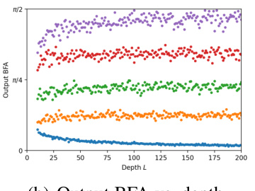
This figure visualizes the Backward-Feature Angle (BFA) at initialization for both MLPs and ResNets. Panel (a) shows that the BFA changes in the initial layers before stabilizing. Panel (b) demonstrates that the BFA at the output layer is independent of depth, but only if β is proportional to 1/√L. Panel (c) shows the relationship between the output BFA and branch scale.

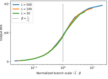
This figure shows the Backward-Feature Angle (BFA) at initialization for Multilayer Perceptrons (MLPs) and Residual Networks (ResNets). Panel (a) demonstrates that the BFA varies initially across layers but stabilizes. Panel (b) illustrates that the output layer’s BFA (θL−1) is largely independent of depth, exhibiting a non-trivial value only when the branch scale (β) is proportional to 1/√L. Finally, panel (c) reveals a direct relationship between the asymptotic output BFA and the normalized branch scale (√L⋅β).

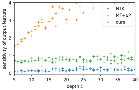
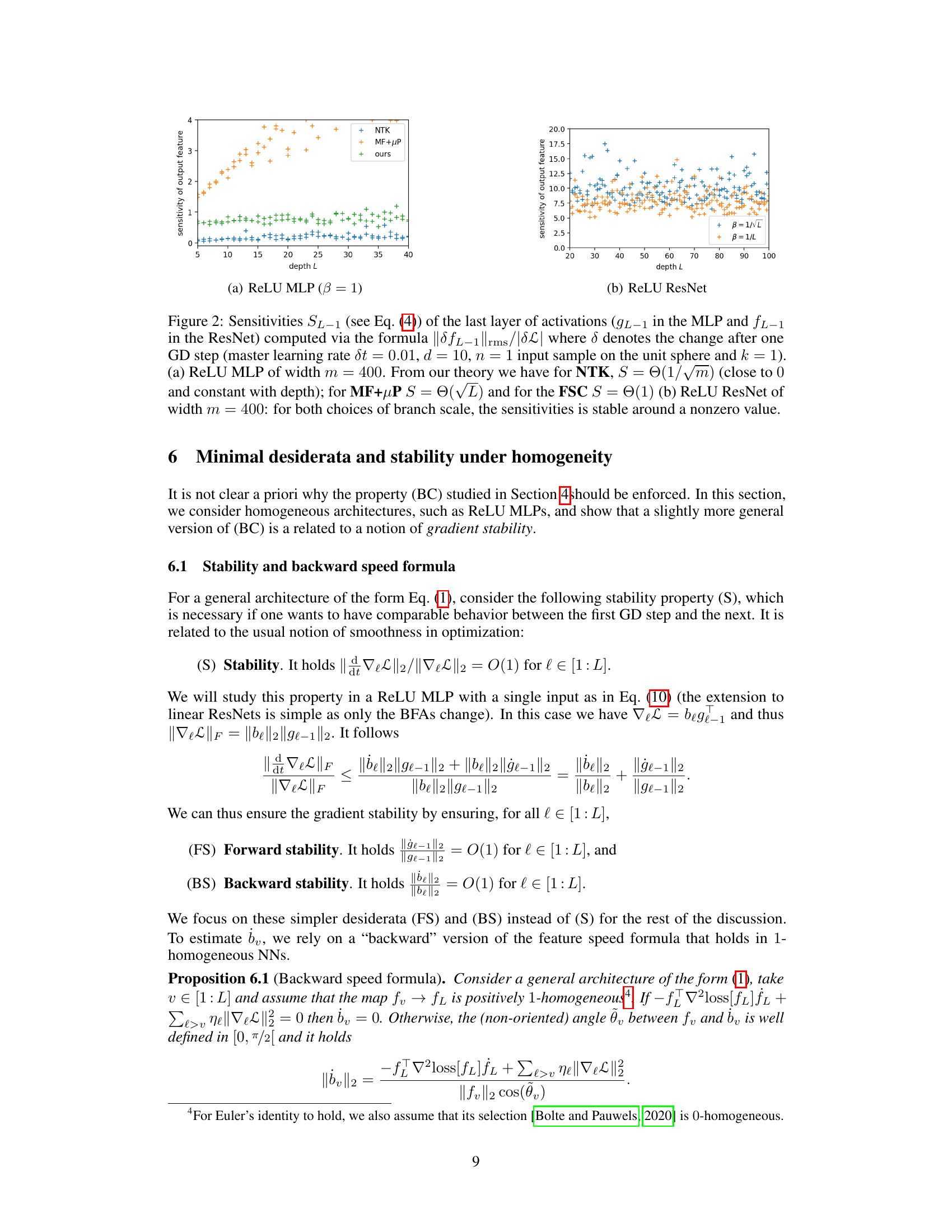
This figure compares the sensitivities of the output feature for three different hyperparameter scalings (NTK, MF+µP, and FSC) across various depths of ReLU MLPs and ReLU ResNets. The sensitivity, represented by S, measures the proportionality between the loss decay and the speed of feature updates. The plots show that the NTK scaling has consistently low sensitivity across depths, whereas MF+µP scaling shows increasing sensitivity with depth. Notably, the FSC scaling maintains stable and relatively constant sensitivity across different depths for both MLPs and ResNets, indicating its potential advantages for controlling training dynamics.

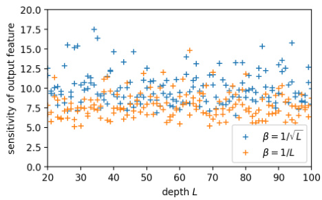
The figure shows the sensitivity of the last layer of activations for ReLU MLP and ReLU ResNet. The sensitivity is computed using the formula ||δfL−1||rms/|SL|, where δ represents the change after one gradient descent step. For the ReLU MLP, the sensitivity is close to 0 for NTK, increases with depth for MF+µP and stays stable around 1 for FSC. For the ReLU ResNet, the sensitivity is stable for both branch scales β=1/√L and β=1/L. This illustrates how different hyperparameter scalings affect the training dynamics of neural networks.

Full paper

#