↗ OpenReview ↗ NeurIPS Homepage ↗ Chat
TL;DR#
Standard graphical models (GMs) can produce biased results, especially when dealing with sensitive attributes or protected groups. This is a significant concern in various fields, as biased GMs can perpetuate existing inequalities and lead to unfair outcomes. The paper highlights this issue, especially in unsupervised learning where fairness is often neglected.
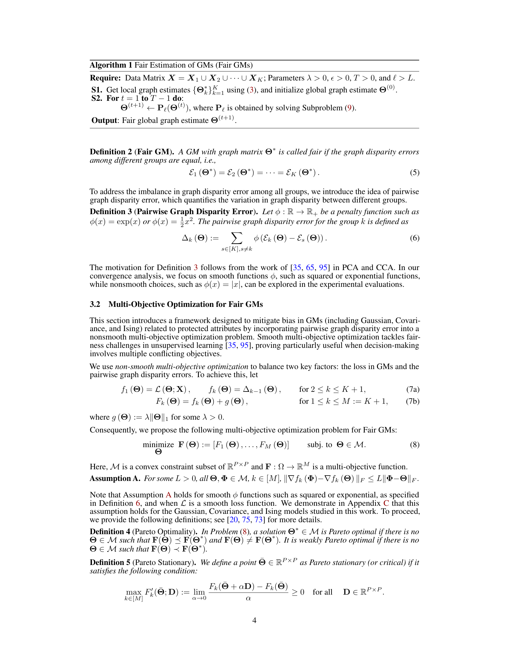
To tackle this, the authors propose a novel framework that incorporates graph disparity error and a specially designed loss function to create a multi-objective optimization problem. This approach strives to balance fairness across different sensitive groups while maintaining the effectiveness of the GMs. The experiments using synthetic and real-world datasets show that the proposed framework effectively reduces bias without impacting the overall performance of the GMs.
Key Takeaways#
Why does it matter?#
This paper is crucial for researchers working on fairness in machine learning, particularly in unsupervised settings. It addresses the often-overlooked issue of bias in graphical model estimation and provides a novel framework for mitigating it. This work is highly relevant given the growing concerns regarding fairness and bias in AI, and opens up new avenues for further research in developing fair and accurate models for various applications.
Visual Insights#

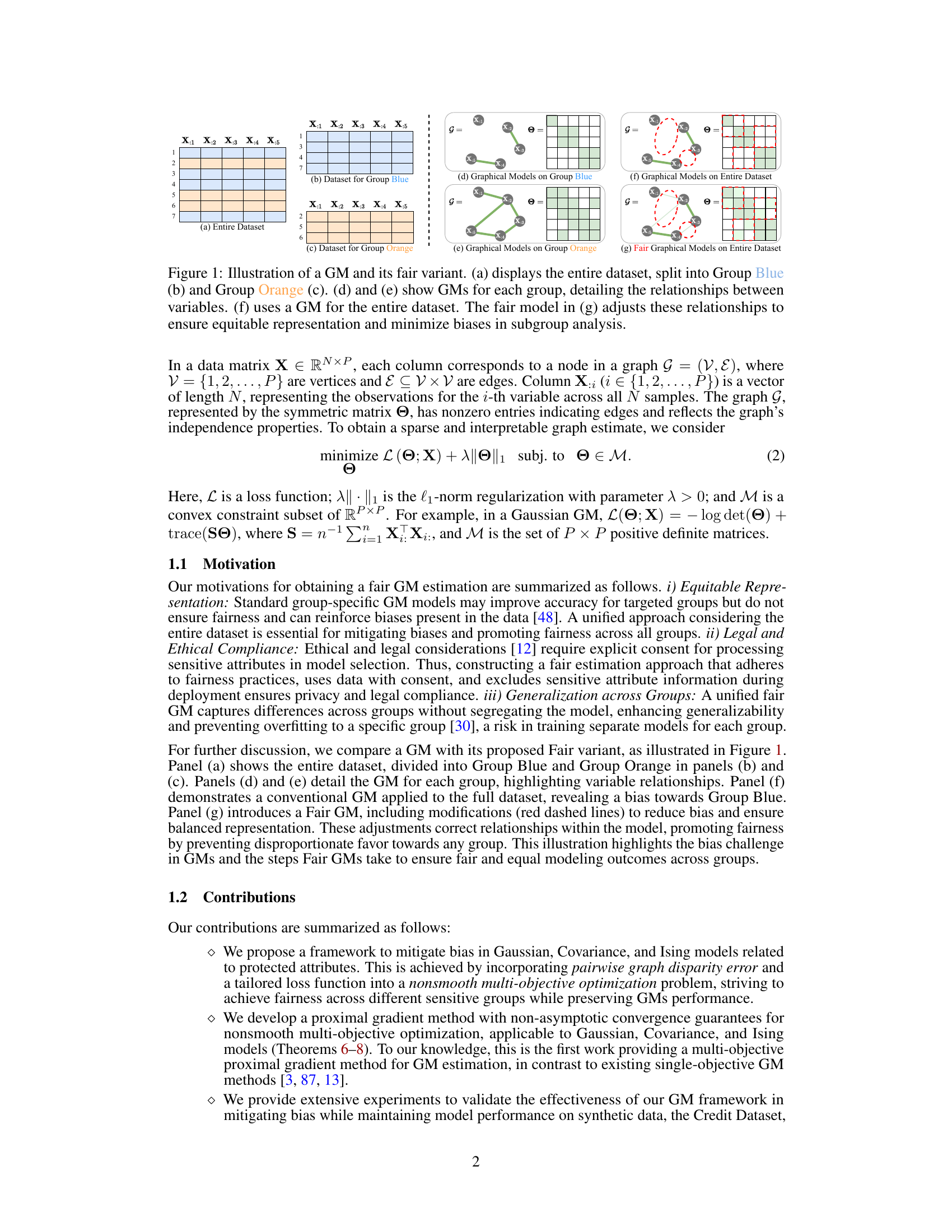
This figure illustrates the concept of fair graphical models. Panel (a) shows the entire dataset split into two groups, blue and orange. Panels (b) and (c) show the datasets for each group separately. Panels (d) and (e) show the graphical models learned for each group individually, highlighting potential biases. Panel (f) displays a graphical model learned on the entire dataset without considering fairness, which may inherit the biases seen in (d) and (e). Finally, panel (g) demonstrates a fair graphical model that addresses these biases by modifying the relationships between variables to ensure more equitable representation across groups.

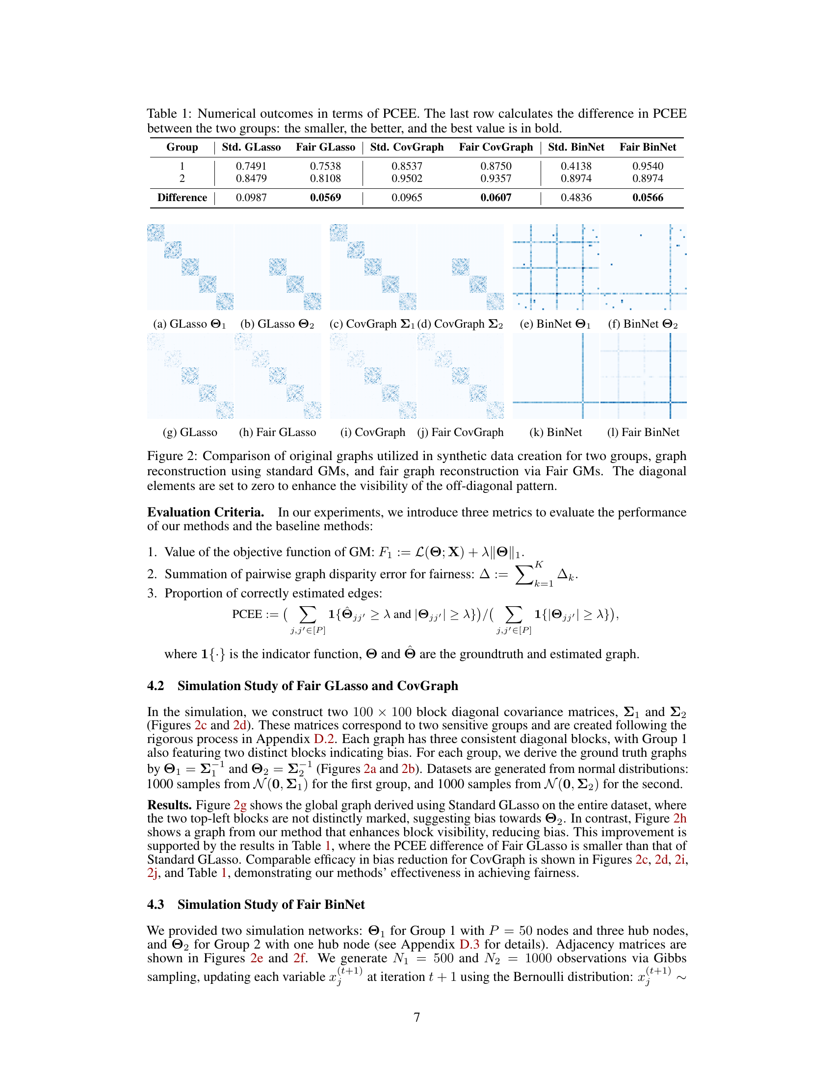
This table presents the Proportion of Correctly Estimated Edges (PCEE) for standard and fair Gaussian graphical models (GLasso), Gaussian covariance graph models (CovGraph), and binary Ising models (BinNet). It shows the PCEE for each model and for two separate groups, along with the difference in PCEE between the groups. A lower difference indicates better fairness.
In-depth insights#
Fair GM Framework#
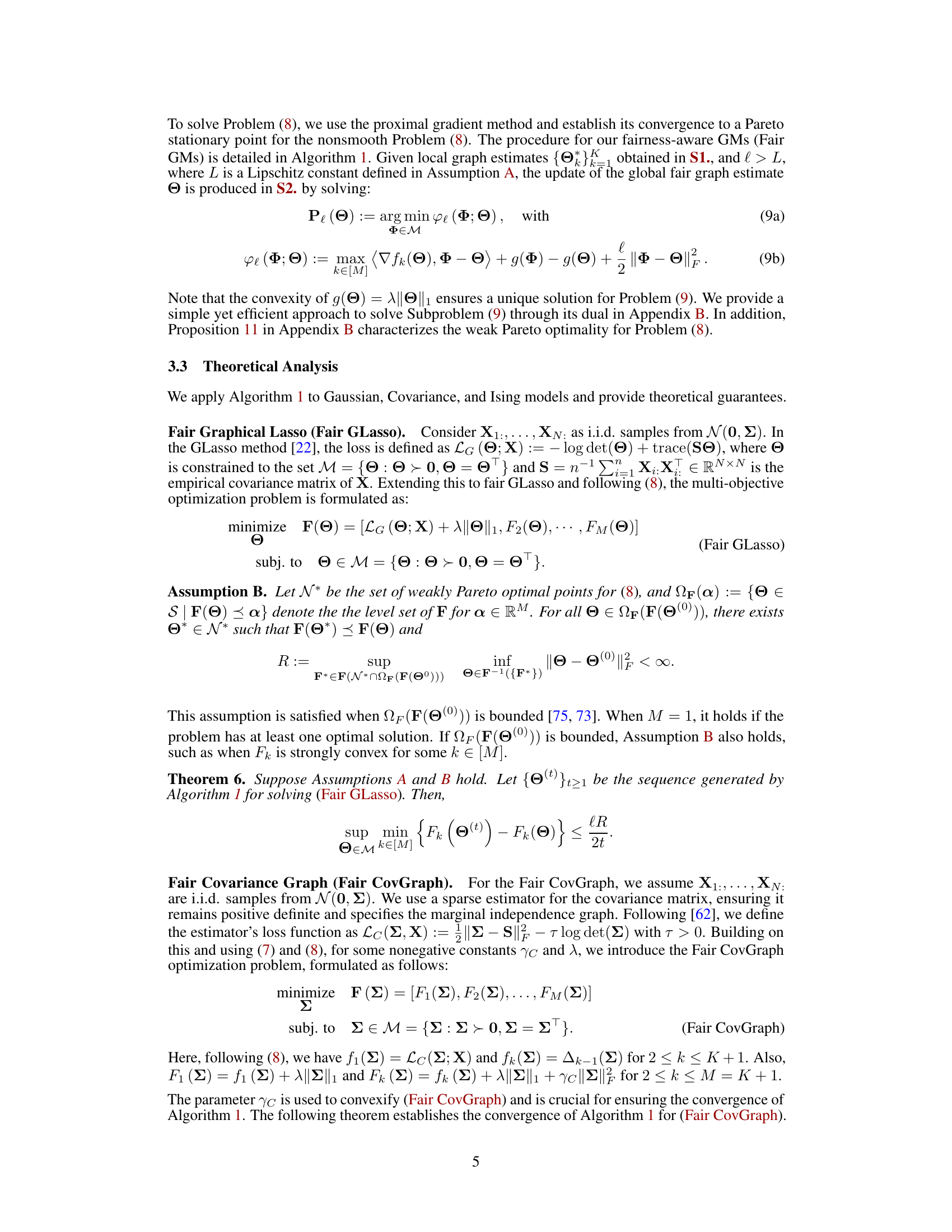
The proposed Fair GM framework tackles the critical issue of bias in graphical model estimation, particularly concerning sensitive attributes. It integrates a novel multi-objective optimization strategy that balances the traditional model accuracy (e.g., minimizing log-likelihood) with a pairwise graph disparity error. This error metric quantifies fairness by measuring the discrepancy in learned relationships across different sensitive groups. The framework’s key innovation lies in simultaneously optimizing for both accurate model representation and equitable treatment of subgroups, mitigating the risk of biased outcomes often associated with standard graphical model approaches. The framework’s broad applicability extends to Gaussian, covariance, and Ising models, and its effectiveness is validated through rigorous experiments demonstrating bias reduction without sacrificing predictive performance. A key contribution is the development of a proximal gradient method with convergence guarantees for solving this nonsmooth multi-objective problem, enhancing both theoretical rigor and practical applicability. However, computational cost remains a limitation, with future work focusing on more efficient optimization strategies and handling larger datasets.
Multi-objective Opt.#
In tackling fairness within graphical models, a multi-objective optimization framework emerges as a crucial element. This approach elegantly addresses the inherent conflict between achieving high model accuracy and ensuring equitable representation across diverse subgroups. Instead of prioritizing a single objective (like minimizing prediction error), it simultaneously considers multiple, potentially competing objectives, such as minimizing prediction error and reducing group-based disparities. This allows for a more nuanced solution that finds a balance between these objectives, rather than sacrificing fairness for accuracy or vice versa. The choice of specific objectives, and the techniques used to balance them (e.g., Pareto optimality, weighted sums), are key aspects influencing the effectiveness and interpretation of the results. The use of this approach showcases a shift from traditional single-objective approaches which often unintentionally amplify existing biases in data. The non-smooth nature of the multi-objective optimization problem further underscores the complexity of balancing fairness and accuracy, necessitating novel, often computationally intensive, optimization strategies.
Proximal Gradient#
Proximal gradient methods are iterative optimization algorithms particularly well-suited for non-smooth optimization problems. They cleverly combine the simplicity of gradient descent with the ability to handle constraints and non-differentiable parts of the objective function via the proximal operator. This operator essentially projects the current iterate onto a set defined by the non-smooth component, ensuring that the algorithm remains within the feasible region. The effectiveness of proximal gradient methods hinges on the choice of a suitable proximal operator and step size, impacting convergence speed and accuracy. For multi-objective problems, as encountered in the paper’s fairness-aware graphical model estimation, proximal gradient methods are particularly valuable because they can effectively balance multiple, potentially conflicting objectives, finding a Pareto optimal solution. The convergence guarantees, often proven through non-asymptotic analysis, provide confidence in the algorithm’s ability to reach a solution within a defined number of iterations, despite the presence of non-smoothness and multiple objectives. Careful tuning of parameters like the step size and regularization parameters is crucial for optimal performance.
Fairness in GMs#
The concept of “Fairness in GMs” (Graphical Models) addresses the crucial issue of bias in the estimation and application of these models. Standard GM procedures can inadvertently amplify biases present in the training data, leading to unfair or discriminatory outcomes. Addressing fairness requires careful consideration of sensitive attributes, such as race or gender, that might be present in the data and could influence the model’s predictions. The challenge lies in developing methods that mitigate these biases without significantly compromising the model’s predictive accuracy or interpretability. This often involves balancing competing objectives: maintaining accurate model performance while simultaneously promoting fairness across different subgroups. Various approaches are explored, such as modifying the loss function to penalize unfair outcomes, incorporating fairness constraints, or using techniques that focus on fair representation of various groups. The effectiveness and efficiency of these methods vary depending on the specific model used and the nature of the data. The implications of achieving fairness in GMs are far-reaching, extending to various applications such as healthcare, finance, and social sciences, where unbiased and equitable model predictions are essential.
Future Directions#
The paper’s exploration of fairness in graphical models opens several exciting avenues for future research. Developing novel group fairness notions that move beyond pairwise disparity, perhaps incorporating intersectional fairness or considering the impact of fairness on downstream tasks, is crucial. The current approach’s sensitivity to loss function selection and objective balancing suggests a need for more robust and adaptable optimization techniques. Exploring alternative optimization methods or developing more sophisticated objective weighting strategies could mitigate this. Extending the framework to different data types beyond Gaussian, covariance, and Ising models (e.g., ordinal data, mixed data types) is important to broaden its applicability and impact. Addressing the computational challenges through more efficient algorithms, parallelization, or approximation techniques is crucial for scalability to larger datasets and more complex models. Finally, empirical evaluations on a wider range of real-world datasets, with a focus on sensitive attributes and diverse demographic groups, will further validate the framework’s effectiveness and identify remaining limitations.
More visual insights#
More on figures
This figure illustrates the difference between standard graphical models (GMs) and fair GMs. It shows how standard GMs can create biased outcomes, particularly when data is split into groups. The fair GM addresses this issue by adjusting the relationships between variables to ensure equitable representation and reduce bias across subgroups.

This figure visually demonstrates the concept of fairness in graphical models (GMs). It shows how standard GMs can produce biased results when applied to datasets with subgroups, and how a fair GM can mitigate this bias by adjusting relationships to ensure equitable representation across subgroups.
This figure illustrates the concept of fairness in graphical models (GMs). Panel (a) shows a dataset split into two groups (blue and orange). Panels (d) and (e) display GMs for each group separately, revealing potential biases in their relationships. Panel (f) shows a GM on the entire dataset, highlighting the effect of these biases. Panel (g) presents a fair GM, which adjusts the relationships to ensure equitable representation across groups. This helps highlight how bias in data can affect GM outcomes and how a fair GM can mitigate these biases.

This figure compares the graphs generated by standard GLasso and Fair GLasso using the ADNI dataset, focusing on the impact of sensitive attributes (marital status and race) on AV45 and AV1451 biomarkers. It visually highlights differences in the network structures produced by each method, demonstrating how Fair GLasso adjusts relationships to mitigate bias.

This figure compares the graphs generated by standard GLasso and Fair GLasso on the ADNI dataset using two different sensitive attributes: marital status (AV45) and race (AV1451). The visualization highlights edges with significant differences in values between the two methods, revealing how Fair GLasso adjusts relationships to mitigate bias and promote equitable representation.

This figure compares brain networks generated using standard GLasso and Fair GLasso on the ADNI dataset. It illustrates how Fair GLasso adjusts relationships to mitigate bias related to sensitive attributes (marital status and race) in amyloid and tau accumulation networks, revealing differences in connectivity patterns.

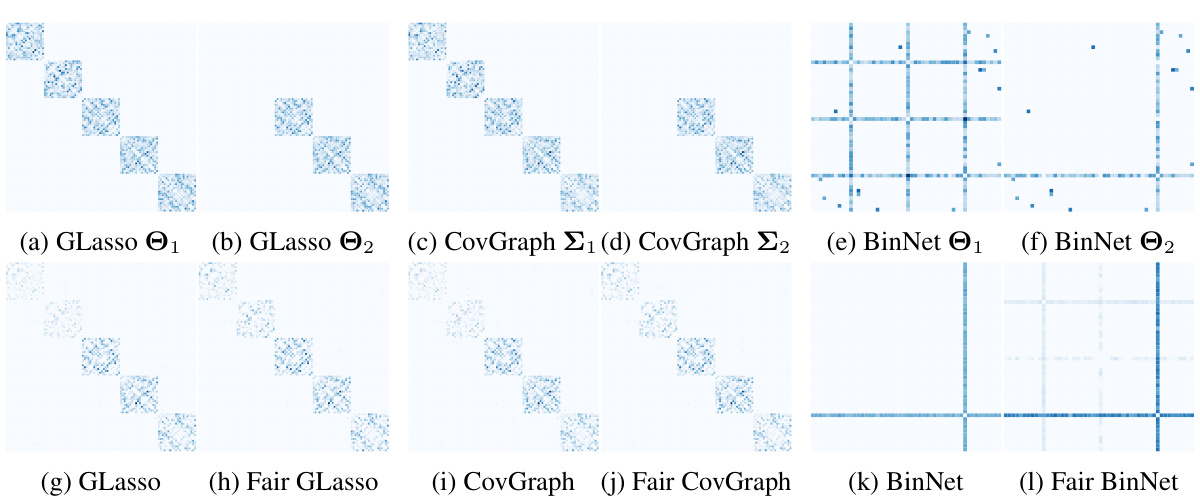
This figure compares the graphical models generated by standard and fair methods across two groups using synthetic data. It shows the true underlying graph structure for each group, the graphical model learned by a standard method applied to each group independently, the graphical model learned by applying the standard method to the combined dataset, and finally the fair graphical model learned by the proposed method on the combined dataset. The diagonal elements are set to zero for better visualization, highlighting the off-diagonal relationships that represent the conditional independence structure of the graph.
This figure visually compares the ground truth graphs for two groups (a, b) with the graphs reconstructed using standard graphical models (c, d, e) and fair graphical models (f, g, h). The zeroing out of diagonal elements improves the visualization of the relationships. The differences highlight how the Fair GM approach mitigates bias and produces more balanced results across both groups.

This figure compares the ground truth graphs for two groups (a, b) with the graphs reconstructed using standard graphical models (c-e) and the fair graphical models (g-l) proposed in the paper. The visualizations clearly show how the standard models fail to capture the differences between the two groups while the fair graphical models better represent the relationships in both groups. The diagonal elements are set to zero to highlight the off-diagonal relationships which represent conditional dependence between variables.

This figure shows a comparison of the results obtained by applying standard graphical models (GMs) and the proposed fair graphical models (Fair GMs) to synthetic data generated for two groups. The left side (a-f) shows the original graphs used to generate the synthetic data and the results from standard GMs, highlighting the difference between the two groups. The right side (g-l) shows the results obtained by Fair GMs. By setting diagonal elements to zero, the off-diagonal patterns become more visible, enhancing the comparison. The figure illustrates how Fair GMs address bias and improve the equitable representation of both groups.
More on tables

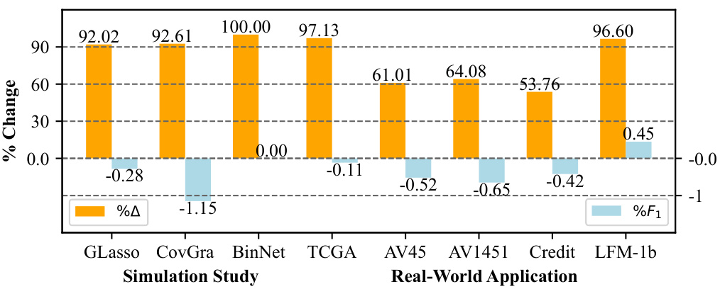
This table presents the performance of the proposed Fair GM framework and the baseline GM method across six different datasets. The metrics include the objective function value (F1), the sum of pairwise graph disparity errors (△), and the computation time. Lower values of F1 and △ indicate better performance, while lower runtime is preferred. The results show that Fair GM generally achieves comparable performance to the baseline GM, while significantly reducing bias, indicated by lower values of △. The runtime is usually longer for Fair GM.

This table presents the results of experiments conducted on four different datasets (Simulation, TCGA, Credit, and LFM-1b) using both standard GMs and Fair GMs. The table compares the standard and Fair versions of GLasso, CovGraph, and BinNet on the objective function value (F1), the sum of pairwise graph disparity error (△), and runtime. Lower values for F1 and △ are better indicating improved performance and fairness, respectively. It shows that the proposed Fair GMs achieve better fairness results without significant performance loss compared to the standard models.

This table presents the results of experiments conducted on two real-world datasets (AV45 and AV1451) using both standard GLasso and the proposed Fair GLasso method. The table compares the objective function value (F1), the pairwise graph disparity error (△), and the runtime for each method across the datasets. Lower values for F1 and △ are preferred, indicating better model performance and fairness. The runtime provides a measure of the computational efficiency of each method.

This table summarizes the performance of the proposed Fair GM framework and compares it against a standard GM on various datasets. The metrics used to evaluate the performance are the objective function value (F1), which measures the model’s fit to the data, the summation of pairwise graph disparity error (△), which quantifies the fairness of the model, and the average computation time. The results show that Fair GM achieves a better balance between model accuracy and fairness.

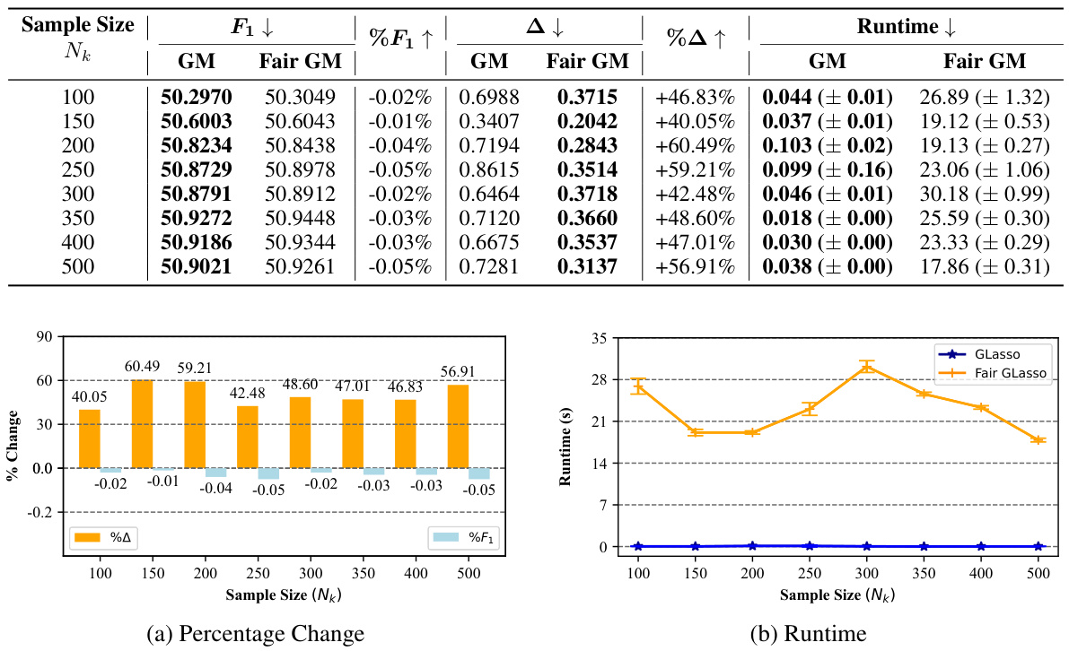
This table presents the results of a sensitivity analysis on the feature size (P) in the GLasso algorithm. For each feature size (from 50 to 400), it shows the objective function value (F1), the pairwise graph disparity error (Δ), and the runtime for both standard GLasso and Fair GLasso. The percentage change in F1 and Δ between the two methods are also included, highlighting the trade-off between fairness and model performance.

This table presents the results of experiments evaluating the performance of the proposed Fair GM framework across various datasets. The metrics used are the objective function value (F1), the pairwise graph disparity error (△), and runtime. Lower values of F1 and △ indicate better performance. Each result is averaged across 10 repeated experiments.

This table presents the results of experiments on several datasets using both standard graphical models (GM) and the proposed Fair GMs. It compares the objective function value (F1), the pairwise graph disparity error (△), and runtime for each method. Lower values for F1 and △ are better, indicating improved model performance and fairness.

This table compares the performance of different optimization algorithms (ISTA, FISTA, PISTA, GISTA, OBN) for both GLasso and MOO in terms of the objective function (F1), pairwise graph disparity error (△), and runtime. It demonstrates the impact of these optimization methods on mitigating bias (indicated by Δ) and maintaining model performance (F1) while improving computational efficiency (runtime). The results are shown for three different synthetic datasets with varying numbers of subgroups, variables and observations.
Full paper#

