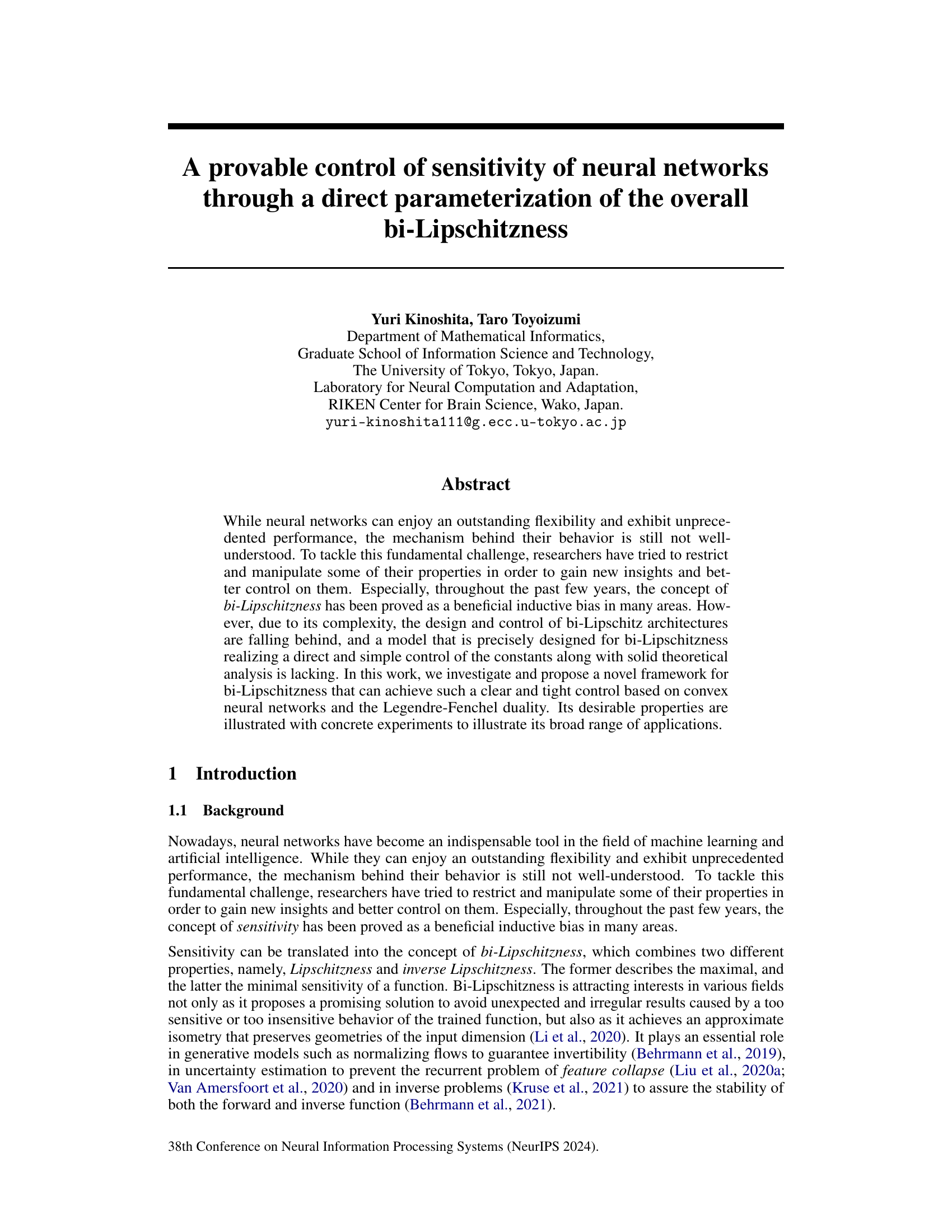
↗ OpenReview ↗ NeurIPS Homepage ↗ Chat
TL;DR#
Neural networks, while powerful, lack interpretability and control over sensitivity. Bi-Lipschitzness, combining Lipschitz and inverse Lipschitz properties, offers a solution but is challenging to implement and control. Existing methods face limitations such as NP-hard constant estimations, difficulty in designing bi-Lipschitz architectures, and complex or loose control over constants. This research introduces a novel framework for building and controlling bi-Lipschitz neural networks using convex networks and Legendre-Fenchel duality. This approach provides theoretical guarantees, direct and tight control over constants, and improved generalization capabilities.
The proposed model, based on convex neural networks and the Legendre-Fenchel duality, provides direct, simple, and tight control of bi-Lipschitz constants via two parameters. It is theoretically guaranteed and demonstrated to be effective. The model’s utility is shown in uncertainty estimation and monotone problem settings. Experiments verify improved performance and tightness of bi-Lipschitz bounds compared to existing methods, highlighting the benefits of direct parameterization.
Key Takeaways#
Why does it matter?#
This paper is crucial for researchers in neural networks and machine learning due to its novel framework for achieving and controlling bi-Lipschitzness in neural networks. This property is increasingly important for applications demanding robust generalization, uncertainty quantification, and handling of inverse problems. The direct parameterization and theoretical guarantees provided offer significant improvements over existing methods. The findings open up new avenues for research, particularly in areas like sensitivity control and inductive bias.
Visual Insights#

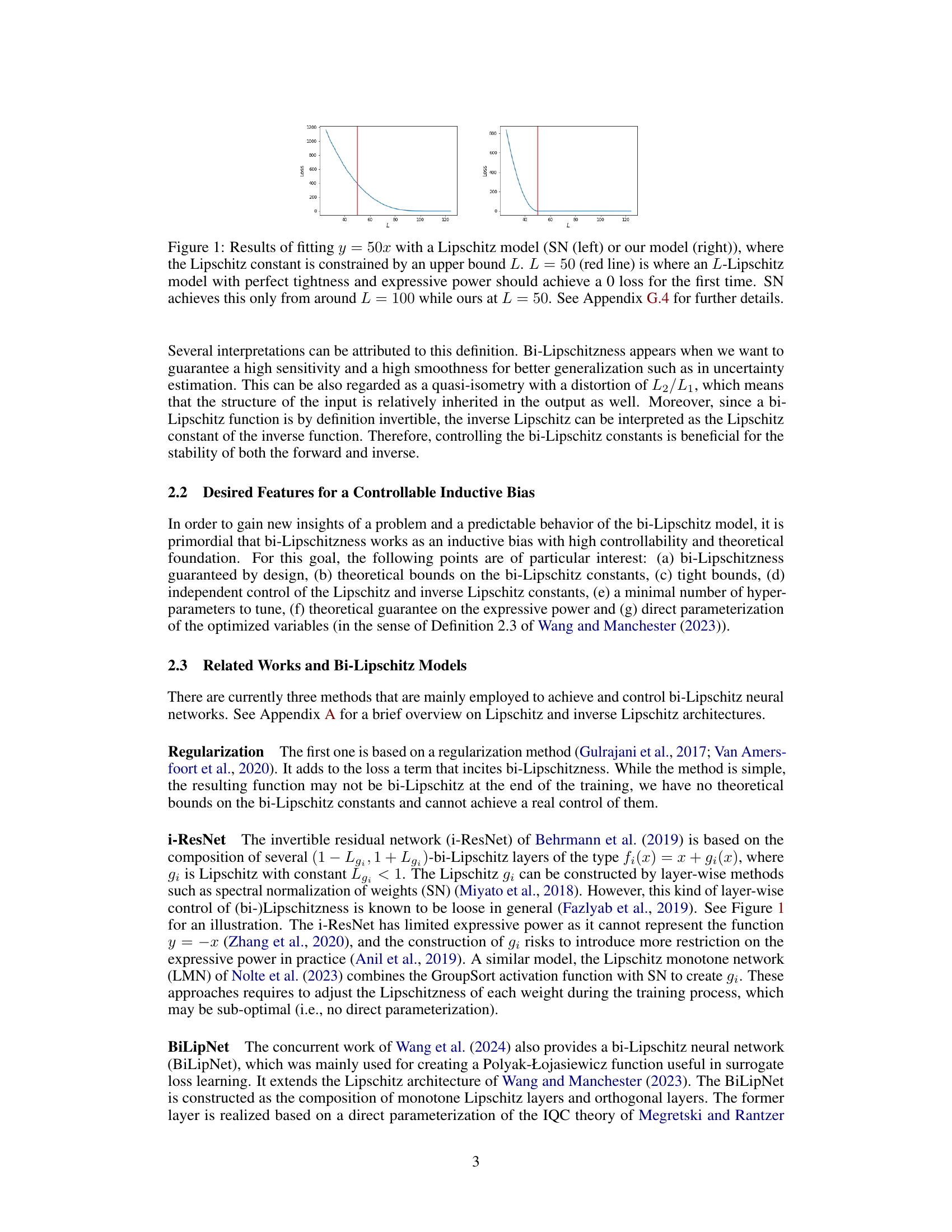
This figure compares the performance of spectral normalization (SN) and the proposed model in fitting a linear function (y = 50x) while constraining the Lipschitz constant (L). The x-axis represents the upper bound of the Lipschitz constant (L), and the y-axis represents the loss. The red line indicates L=50, where a perfectly tight and expressive L-Lipschitz model should achieve zero loss. The plot demonstrates that the proposed model achieves zero loss at L=50, showcasing its superior tightness and expressive power, while SN only reaches zero loss when L is significantly higher (around 100).

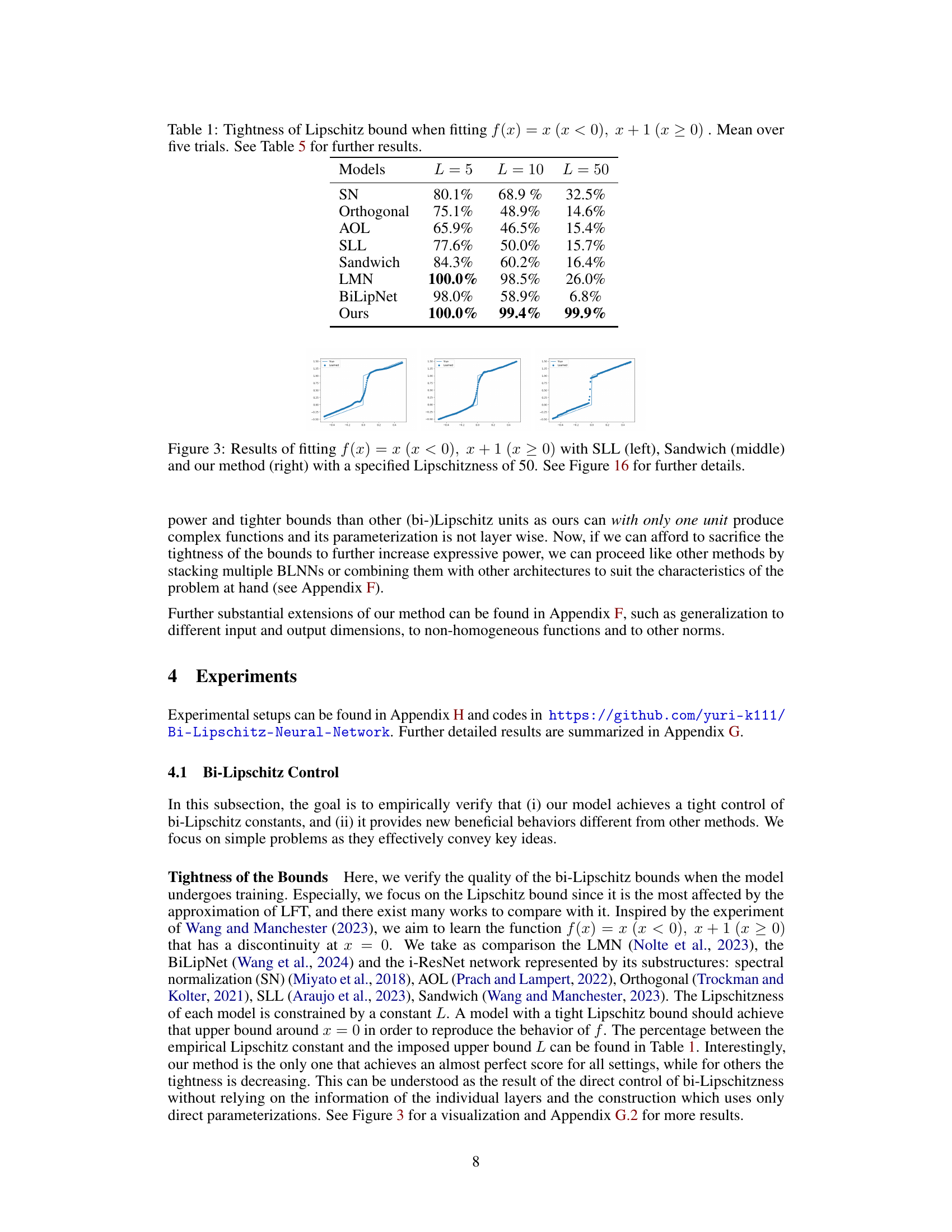
This table compares the tightness of the Lipschitz bound achieved by different models when fitting a piecewise linear function with a discontinuity. The models are tested with different upper bounds (L) on the Lipschitz constant. Tightness is measured as the percentage difference between the imposed Lipschitz constant and the actual Lipschitz constant observed after training. The table shows that the proposed method (Ours) achieves much tighter bounds, particularly at higher values of L, indicating better control over the Lipschitzness.
In-depth insights#
Bi-Lipschitz Control#
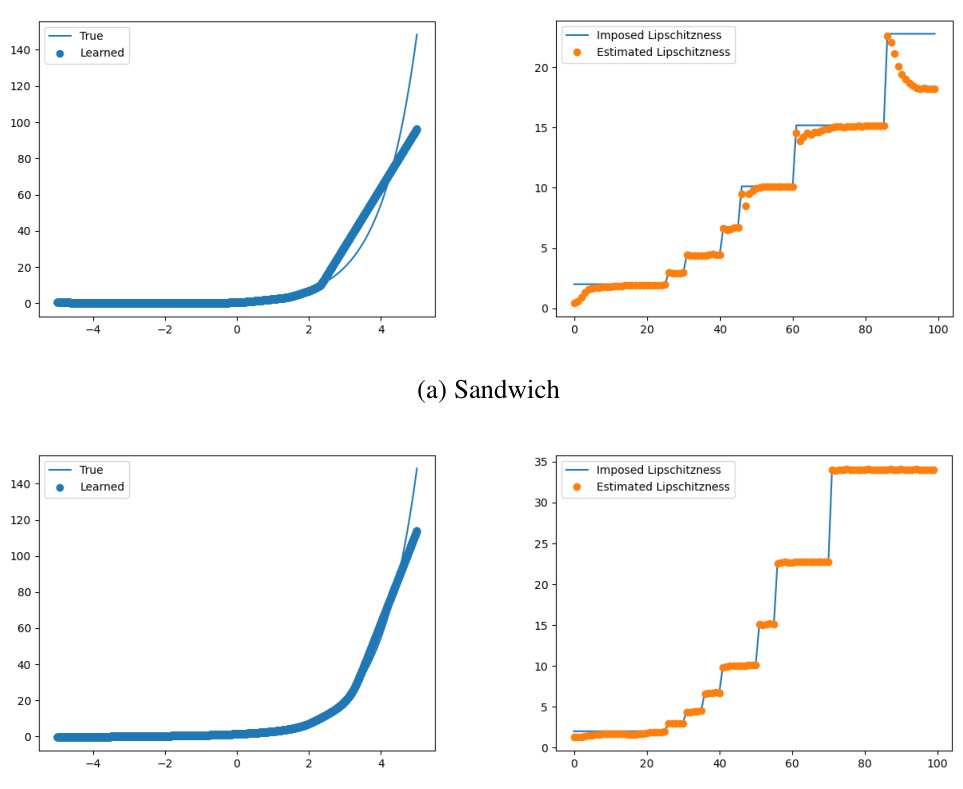
The section on “Bi-Lipschitz Control” in this research paper is crucial because it demonstrates the effectiveness of the proposed bi-Lipschitz neural network (BLNN) model. The experiments presented highlight the model’s ability to tightly control bi-Lipschitz constants, a significant improvement over existing methods. This precise control is shown through experiments involving fitting functions with discontinuities and demonstrating that the BLNN consistently achieves near-perfect accuracy in maintaining the imposed Lipschitz bound. Furthermore, the results showcase the model’s flexibility in handling various Lipschitz regimes, accurately fitting functions even when the specified Lipschitz constant is underestimated or overestimated, unlike layer-wise methods which struggle under such conditions. This signifies a crucial advantage for BLNN in scenarios requiring robust control over function sensitivity and generalization capabilities. The ability to manipulate Lipschitz and inverse Lipschitz constants independently shows a better understanding of the nuanced relationship between these two concepts, leading to a more predictable and controllable inductive bias.
BLNN Architecture#
The Bi-Lipschitz Neural Network (BLNN) architecture is novel in its design, directly parameterizing the overall bi-Lipschitz property of the network via the Legendre-Fenchel transformation. This approach differs significantly from layer-wise methods, providing a more direct and tight control over the Lipschitz and inverse Lipschitz constants using only two parameters. The architecture leverages the properties of convex neural networks, ensuring theoretical guarantees on bi-Lipschitzness. Furthermore, the use of Legendre-Fenchel duality offers computational efficiency, reducing the need to track the whole forward pass during backpropagation. The framework’s expressive power is notable, allowing approximation of complex bi-Lipschitz functions and extending to partially bi-Lipschitz variants for increased scalability and flexibility. Overall, theoretical guarantees and effective control are key strengths of the BLNN architecture, offering a significant advancement in designing and manipulating bi-Lipschitz neural networks.
Uncertainty Estimator#
The concept of an ‘Uncertainty Estimator’ within the context of neural networks is crucial for building reliable and trustworthy AI systems. A robust uncertainty estimator should accurately quantify the confidence of a model’s predictions, distinguishing between genuine uncertainty (due to noise or inherent randomness in the data) and epistemic uncertainty (due to limitations in the model’s knowledge). This is especially important in high-stakes applications like medical diagnosis or autonomous driving where miscalibration could have severe consequences. Effective uncertainty estimation often involves techniques that go beyond simple prediction probabilities, incorporating methods such as deep ensembles, Bayesian neural networks, or more recent approaches like Deterministic Uncertainty Quantification (DUQ). The choice of method depends on the specific application and the trade-off between accuracy and computational cost. Bi-Lipschitz neural networks, as explored in this research, offer a novel perspective by imposing constraints on the model’s sensitivity and invertibility, potentially leading to more reliable uncertainty quantification. However, the effectiveness of any method is contingent upon a comprehensive understanding of the data and model limitations, requiring careful validation and testing.
Monotone Settings#
The section on “Monotone Settings” explores the application of the proposed bi-Lipschitz neural network model to machine learning problems exhibiting monotone behavior. This is a significant contribution as many real-world datasets show inherent monotonic relationships between features and target variables. The authors demonstrate that incorporating this inductive bias into the model architecture leads to improved generalization performance and efficiency compared to existing state-of-the-art monotone models. They validate this claim through experiments on benchmark datasets known to possess such monotone properties, highlighting the model’s ability to leverage this structural information for improved prediction accuracy. This showcases a practical advantage of the proposed framework and further underscores its versatility. The results emphasize the importance of carefully considering the underlying structure of a dataset when selecting or designing a model, thus contributing to a more effective and insightful approach to machine learning model development.
Future Directions#
Future research could explore several promising avenues. Improving the efficiency and scalability of the proposed bi-Lipschitz neural network (BLNN) is crucial, perhaps through exploring more efficient optimization techniques for the Legendre-Fenchel transformation or developing approximate methods that maintain theoretical guarantees. Extending the framework to handle more complex architectures such as those with skip connections, residual blocks, and attention mechanisms would broaden its applicability. Another key direction is investigating the theoretical underpinnings of bi-Lipschitzness as an inductive bias and its connection to generalization, robustness, and uncertainty quantification. Empirical studies could delve into the expressive power of BLNN compared to other bi-Lipschitz models, especially in scenarios with high dimensionality and complex relationships. Finally, applying BLNN to diverse machine learning tasks, such as those requiring robustness to adversarial attacks, monotone modeling, or uncertainty estimation, will reveal its practical effectiveness and potential.
More visual insights#
More on figures

This figure compares the computational complexity (FLOPS and memory usage) of a single iteration for different neural network architectures. It compares a traditional feedforward network against several variations of the proposed Bi-Lipschitz Neural Network (BLNN). Specifically, it shows the complexity for a BLNN using the full backpropagation method, a BLNN using Theorem 3.7 for optimized backpropagation, and a partially bi-Lipschitz BLNN (PBLNN). The results are displayed as graphs showing the FLOPS (floating point operations per second) and memory usage in MB (megabytes) as functions of batch size (number of data samples processed simultaneously). The BLNN variants show varying levels of complexity improvement over the traditional feedforward network, demonstrating the computational efficiency of the proposed methods, particularly when using the optimized backpropagation technique (Theorem 3.7).

This figure compares the performance of three different bi-Lipschitz models (SLL, Sandwich, and the proposed model) on fitting a piecewise linear function with a specified Lipschitz constant of 50. The left column shows the fitted curve over the whole range of the input data. The right column zooms into the area around the discontinuity to highlight the differences in the accuracy of fitting the function, especially in regions where the Lipschitz constraint is binding.

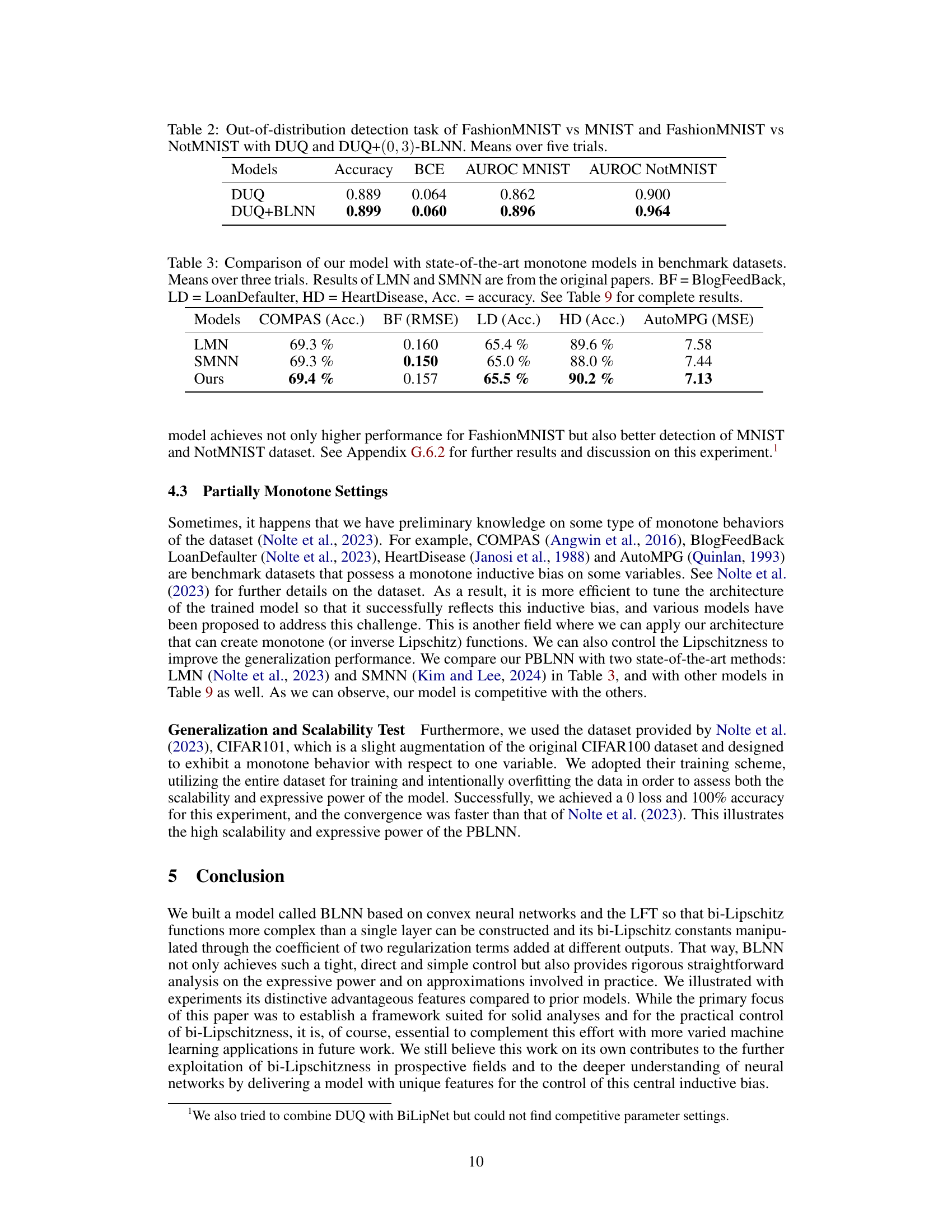
This figure compares the uncertainty estimation results of several models on the two moons dataset. The models compared include a deep ensemble, DUQ without regularization, DUQ, and DUQ combined with the proposed Bi-Lipschitz neural network (BLNN) with varying parameters α and β. The color represents the level of uncertainty, with blue indicating high uncertainty and yellow indicating low uncertainty. The figure visually demonstrates the improvement in uncertainty estimation that the BLNN provides compared to existing methods.
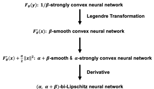
This figure illustrates the process of constructing a bi-Lipschitz neural network using the Legendre-Fenchel transformation and the Brenier map. It starts with a 1/β-strongly convex neural network, applies the Legendre transformation to obtain a β-smooth convex network, then adds a term to make it α + β-smooth and α-strongly convex. Finally, taking the derivative results in an (α, α + β)-bi-Lipschitz neural network.
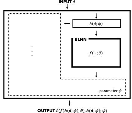
This figure shows a generalized architecture that includes the proposed Bi-Lipschitz neural network (BLNN) model. The input data (d) is first processed by a function h(d; φ) parameterized by φ. The output of h(d; φ) is then fed into the BLNN, f(-; θ), which is parameterized by θ. The BLNN’s output is further processed by a loss function L parameterized by ψ, which produces the final output. This architecture demonstrates the flexibility of integrating the BLNN into more complex models.

This figure shows the evolution of the Lipschitz and inverse Lipschitz constants throughout the optimization process for three different algorithms: Gradient Descent (GD), Accelerated Gradient Descent (AGD), and the Newton method. Each row represents a different optimization algorithm, with the left column showing the Lipschitz constant and the right column showing the inverse Lipschitz constant. The x-axis represents the number of iterations, while the y-axis represents the value of the Lipschitz (or inverse Lipschitz) constant. The plots illustrate how well each algorithm maintains the bi-Lipschitz property (i.e., the Lipschitz and inverse Lipschitz constants remain relatively stable and close to their theoretical bounds) during the optimization. The red line indicates the true value of the constants.

The figure shows the evolution of Lipschitz and inverse Lipschitz constants during the training process using three different optimization algorithms: Gradient Descent (GD), Accelerated Gradient Descent (AGD), and Newton’s method. Each algorithm’s performance is shown in a separate row of the figure with plots showing both the estimated and true values over the iterations. This visualization helps in understanding the effectiveness of various optimization strategies in maintaining bi-Lipschitz properties throughout the training.

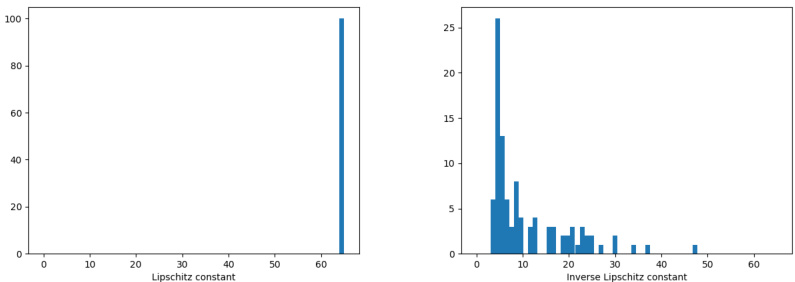
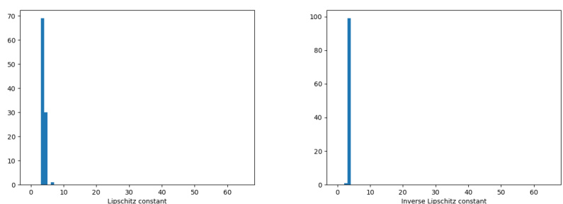
This figure shows the estimated Lipschitz and inverse Lipschitz constants obtained from a BLNN model using gradient descent with softplus activation functions. Two separate plots are shown: one for a network with 3 hidden layers, and another for a network with 10 hidden layers. The x-axis represents different values of β (beta), calculated as β = 0.05 + 99.95*j/100 where j is an index. The plots visually represent the relationship between the calculated Lipschitz and inverse Lipschitz constants and different values of beta, demonstrating how the model’s sensitivity (as measured by these constants) changes with varying beta values. The ‘Lower bound’ and ‘Upper bound’ lines indicate the theoretically expected range of these constants based on the model parameters and design.
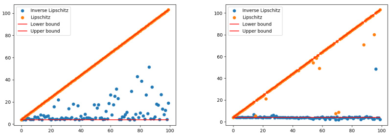
This figure shows the estimated Lipschitz and inverse Lipschitz constants obtained from a BLNN model using gradient descent with softplus activation functions. The x-axis represents a parameter β, which varies from 0.05 to 100. Two sets of results are displayed: one with a network architecture of 3 hidden layers and another with 10 hidden layers. The plots visualize the relationship between the parameter β and the resulting Lipschitz and inverse Lipschitz constants, providing empirical evidence of how the model’s sensitivity (as measured by the Lipschitz constants) is controlled through the parameter β. The lines show theoretical bounds, illustrating that the empirically obtained values stay within the theoretical expectations.
This figure compares the performance of spectral normalization (SN) and the proposed bi-Lipschitz model in fitting a linear function (y = 50x) with a constrained Lipschitz constant (L). The plot shows that the proposed model achieves zero loss at the theoretical minimum L=50, while SN only achieves zero loss at a much larger L=100, demonstrating the improved tightness and expressive power of the proposed model.
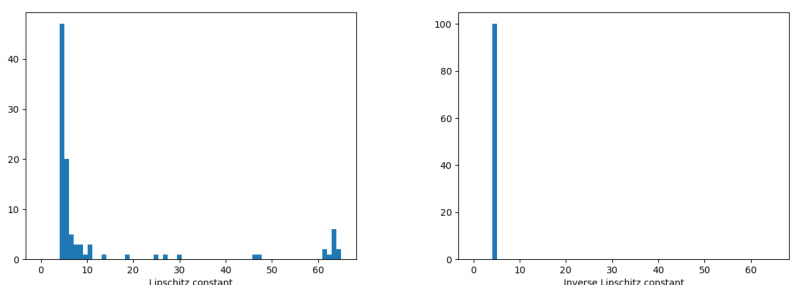
This figure shows the estimated Lipschitz and inverse Lipschitz constants obtained from 100 different (4, β)-BLNNs, where β varies from 0.05 to 100. The experiments were conducted using gradient descent with softplus activation functions. The left panel displays results with 3 hidden layers, while the right panel shows results for 10 hidden layers. The x-axis represents the value of β, showcasing how the estimated Lipschitz and inverse Lipschitz constants change with different β values.
This figure compares the performance of spectral normalization (SN) and the proposed bi-Lipschitz model in fitting the linear function y = 50x. The x-axis represents the upper bound (L) on the Lipschitz constant. The y-axis represents the loss. The red line indicates where a perfectly tight and expressive L-Lipschitz model should achieve zero loss. The results show that the proposed model achieves zero loss at L=50, while SN only achieves it at approximately L=100, demonstrating the superior tightness and expressiveness of the proposed model.
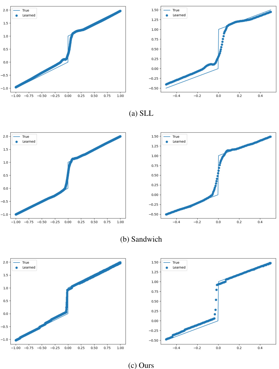
This figure compares the results of fitting a piecewise linear function using three different methods: SLL, Sandwich, and the proposed method. Each method is constrained to have a Lipschitz constant of 50. The plots show that the proposed method achieves a significantly better fit of the function, especially around the discontinuity at x = 0. The zoomed-in plots on the right emphasize the superior accuracy of the proposed method in capturing the sharp transition near the discontinuity.

This figure compares the performance of spectral normalization (SN) and the proposed model in fitting a linear function (y = 50x) with a Lipschitz constraint. The x-axis represents the Lipschitz bound (L), and the y-axis represents the loss. The red line indicates the point where a perfectly tight L-Lipschitz model should achieve zero loss. The proposed model achieves this at L ≈ 50, demonstrating better control and tightness of the Lipschitz constraint compared to SN which only achieves it at L ≈ 100.
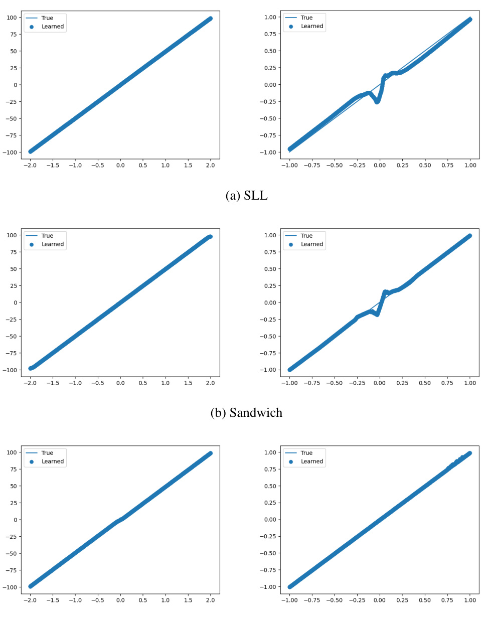
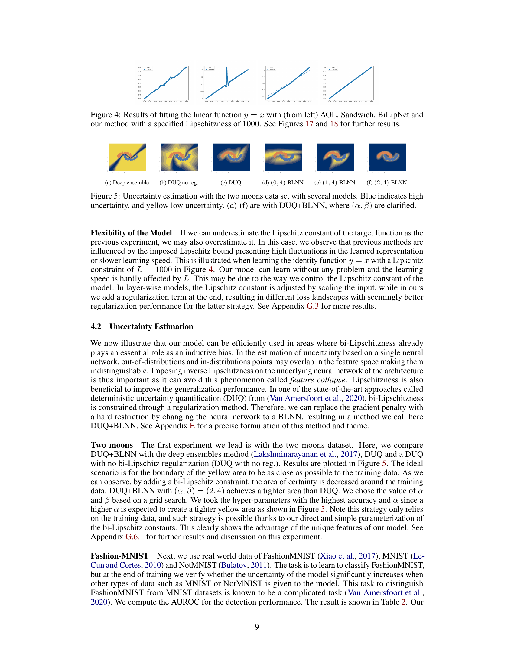
This figure shows the results of fitting a piecewise linear function (y=x for x<0 and y=x+1 for x>=0) using three different bi-Lipschitz models: SLL, Sandwich, and the proposed model. Each model is trained with a Lipschitz constraint of 50. The left column plots the entire range of the fitted curve against the true function, while the right column zooms in on the region near the discontinuity (x=0) to highlight the differences in the models’ behavior near the transition point. The proposed method demonstrates a much tighter fit to the true function, especially near the discontinuity. This indicates a superior ability to control and maintain the bi-Lipschitz property throughout the training process, compared to the layer-wise approaches of SLL and Sandwich.
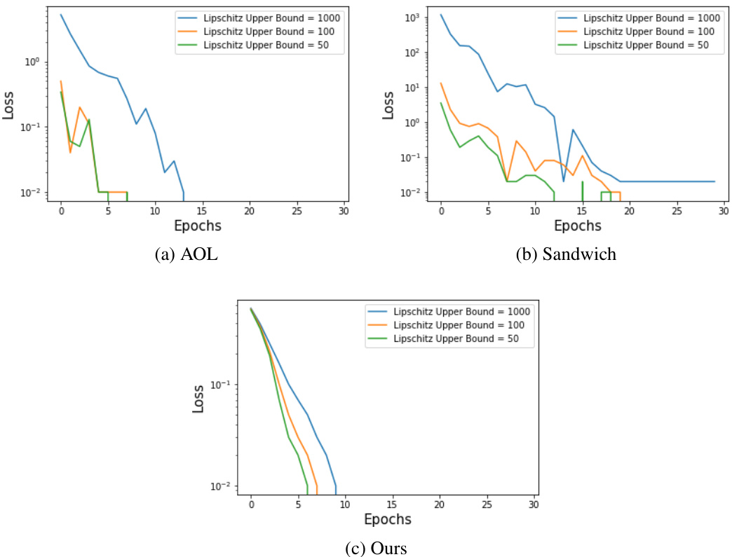
This figure compares the performance of spectral normalization (SN) and the proposed model in fitting a linear function y = 50x, with the Lipschitz constant constrained by an upper bound L. The plot shows the loss as a function of L. The proposed model achieves a loss of 0 at L=50, demonstrating perfect tightness and expressive power, while the SN model only achieves this at a much larger L=100, indicating less tightness and expressive power.
This figure compares the performance of spectral normalization (SN) and the proposed bi-Lipschitz model in fitting a linear function (y = 50x). The x-axis represents the upper bound (L) on the Lipschitz constant, and the y-axis shows the loss. The red line indicates the expected loss (0) when the model achieves perfect tightness and expressive power at L=50. The proposed model achieves a loss near zero at L=50, demonstrating tight control of the Lipschitz constant. In contrast, the SN model only reaches a loss near zero at a significantly higher L value (around 100), indicating looser control. This highlights the improved performance of the proposed model in precisely controlling bi-Lipschitzness.

This figure shows the results of fitting the linear function y = 50x using two different Lipschitz models: a spectral normalized (SN) model and the proposed model in the paper. The x-axis represents the upper bound L imposed on the Lipschitz constant, and the y-axis shows the loss achieved by the model. The red line indicates the point where a perfectly tight and expressive L-Lipschitz model should achieve zero loss (L=50). The plot highlights the superior performance of the proposed model, which achieves zero loss at L=50, while the SN model only reaches zero loss at around L=100. This demonstrates that the proposed model offers tighter control over the Lipschitz constant compared to the existing SN approach.
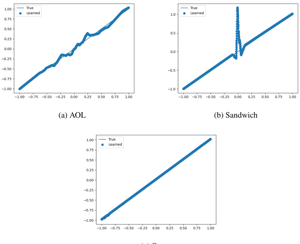
This figure compares the performance of three different bi-Lipschitz models in fitting a curve with a specified Lipschitz constant of 50. The models compared are the Spectral Lipschitz Layer (SLL), the Sandwich layer, and the proposed model from the paper. The results are visualized by plotting the learned curve and showing the fit next to the true curve. The rightmost column of subplots shows a zoomed-in view of the rightmost columns, highlighting the details of how well each model fits the curve. The figure demonstrates that the proposed method outperforms the other models.
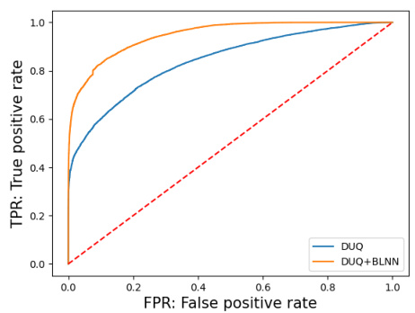
This figure shows the Receiver Operating Characteristic (ROC) curves for out-of-distribution detection experiments using the DUQ and DUQ+BLNN models. The left plot shows the results for distinguishing FashionMNIST from MNIST, while the right plot shows the results for distinguishing FashionMNIST from NotMNIST. The ROC curves illustrate the trade-off between the true positive rate (TPR) and the false positive rate (FPR) for both models, indicating their performance in identifying out-of-distribution samples. The downsampled data used in this experiment consisted of images reduced in size from 28x28 to 14x14 via max pooling.
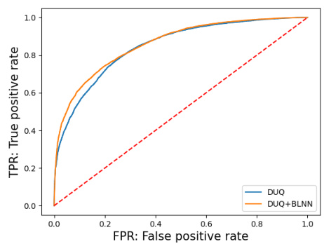
This figure shows the Receiver Operating Characteristic (ROC) curves for the out-of-distribution detection task on the Fashion-MNIST dataset. Two scenarios are presented: Fashion-MNIST vs. MNIST and Fashion-MNIST vs. NotMNIST. A downsampled version of the Fashion-MNIST dataset (14x14) is used. The curves compare the performance of the DUQ model (blue) and the DUQ+BLNN model (orange). The diagonal dashed line represents random chance; models above the line demonstrate better-than-chance performance in distinguishing between in-distribution and out-of-distribution samples. The area under the curve (AUC) is a common metric that quantifies performance.

This figure compares the uncertainty estimation performance of different models on the two moons dataset. It shows uncertainty maps, where blue indicates high uncertainty and yellow indicates low uncertainty. The models compared include Deep Ensembles, DUQ without regularization, DUQ (with regularization), and DUQ+BLNN with different (α, β) parameters. DUQ+BLNN is the proposed method of the paper, which incorporates the bi-Lipschitz Neural Network (BLNN). The comparison highlights how the proposed method, with its controlled bi-Lipschitzness, leads to better uncertainty estimates.

This figure shows the uncertainty quantification of the two moons dataset using the DUQ+BLNN model with a high alpha (α = 5.0) and beta (β = 30.0). The points are not shown to emphasize the area of high certainty (yellow). The high alpha value causes the model to be highly uncertain almost everywhere except for a small region near the training data. This highlights how the parameters α and β can be used to control the level of uncertainty in the model’s predictions.
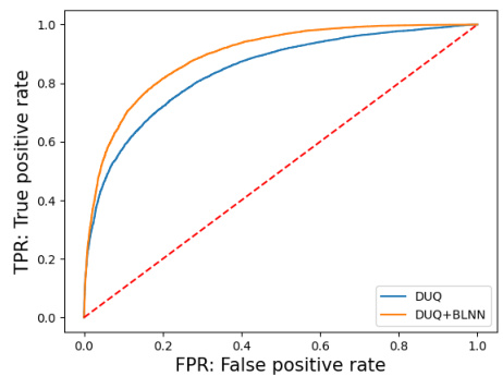
This figure shows the Receiver Operating Characteristic (ROC) curves for the out-of-distribution detection task. The left panel displays the ROC curve for distinguishing FashionMNIST from MNIST, while the right panel shows the ROC curve for distinguishing FashionMNIST from NotMNIST. The ROC curves compare the performance of the standard DUQ model against the DUQ+BLNN model, illustrating the improvement in detection performance achieved by incorporating the bi-Lipschitz neural network.
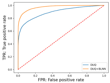
This figure shows the Receiver Operating Characteristic (ROC) curves for the out-of-distribution detection task using the DUQ and DUQ+BLNN models. The left panel displays the ROC curve when distinguishing between FashionMNIST and MNIST datasets, while the right panel shows the ROC curve for distinguishing between FashionMNIST and NotMNIST datasets. The ROC curves illustrate the trade-off between the true positive rate (TPR) and the false positive rate (FPR) for both models, allowing for a comparison of their performance in detecting out-of-distribution samples. The dashed line represents the performance of a random classifier. The DUQ+BLNN model generally performs better, showing higher TPR for the same FPR.

Uncertainty quantification results for the two moons dataset using the DUQ+BLNN model with varying alpha values (α = 0.0, 1.0, and 2.0). The plots show the uncertainty estimation, where blue indicates high uncertainty and yellow indicates low uncertainty. The figure visually demonstrates how different alpha values influence the uncertainty estimation.
More on tables
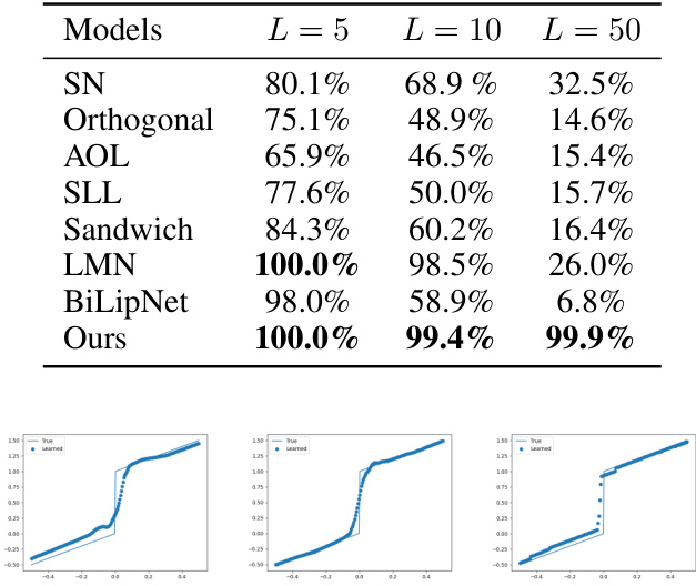
This table presents the results of an experiment designed to evaluate the tightness of the Lipschitz bound achieved by several Bi-Lipschitz models when fitting a piecewise linear function. The models were trained with different upper bounds on the Lipschitz constant (L=5, 10, 50). The table shows the percentage of times each model’s actual Lipschitz constant (after training) fell within a certain percentage of the imposed upper bound L. A higher percentage indicates better tightness of the bound, meaning the model’s actual Lipschitz constant remained closer to the constrained value. The results are averaged over five trials.

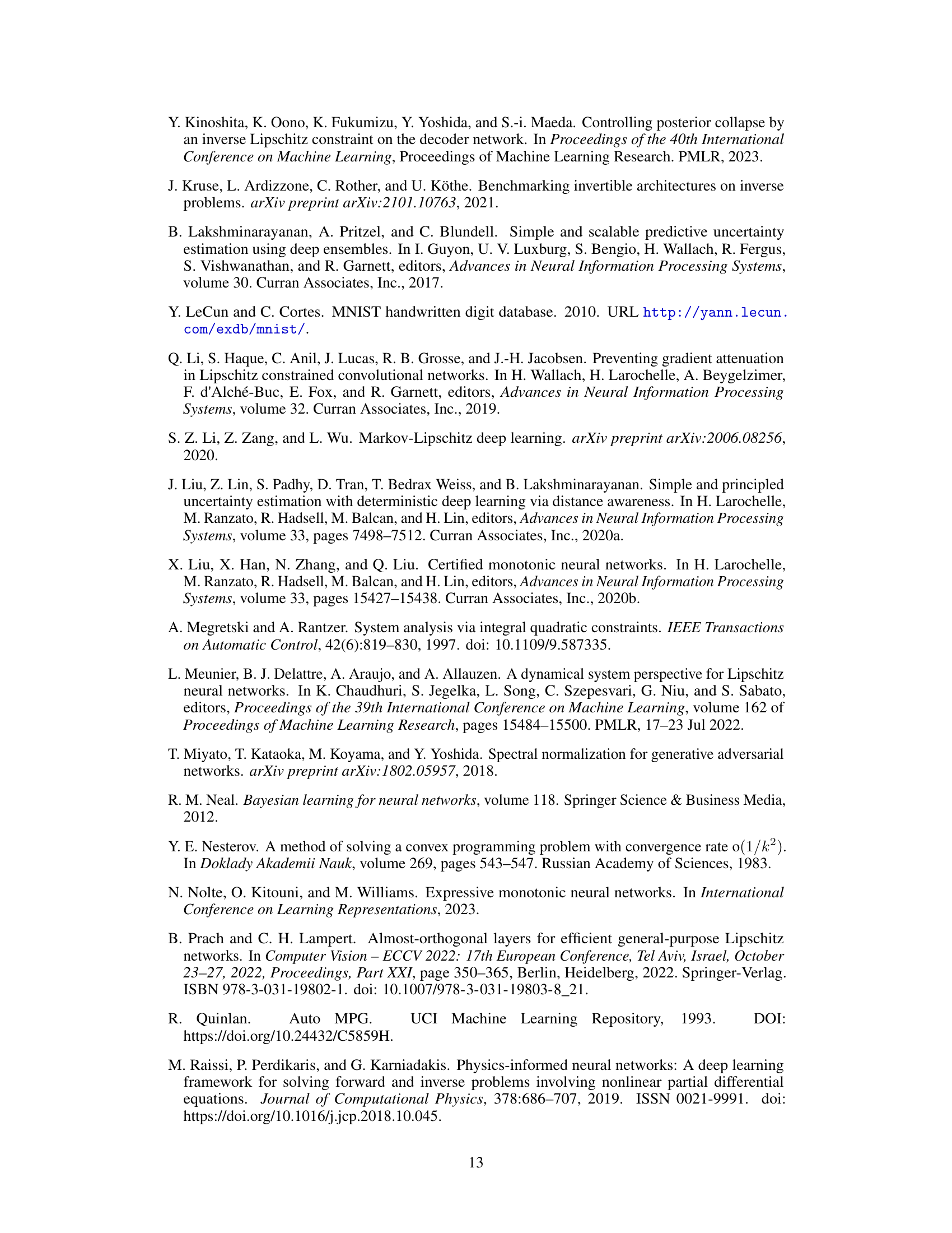
This table presents the results of an out-of-distribution detection experiment comparing the performance of DUQ (Deep Uncertainty Quantification) and DUQ+BLNN (DUQ enhanced with the Bi-Lipschitz Neural Network) on two tasks: distinguishing FashionMNIST from MNIST, and FashionMNIST from NotMNIST. The results show accuracy, binary cross-entropy (BCE) loss, and Area Under the Receiver Operating Characteristic curve (AUROC) for each model and dataset. The data demonstrates that the addition of the BLNN improves performance on the out-of-distribution detection task.

This table compares the performance of the proposed Bi-Lipschitz neural network model against state-of-the-art monotone models on several benchmark datasets. The metrics used for comparison include accuracy (Acc.), Root Mean Squared Error (RMSE), and Mean Squared Error (MSE), depending on the nature of each dataset. The results show that the proposed model achieves competitive or better performance than the existing methods.

This table presents the results of an out-of-distribution detection task comparing the performance of two models: DUQ and BLNNconv then DUQ. The dataset used is CIFAR10 for in-distribution data and SVHN for out-of-distribution data. The table shows the accuracy, loss, and AUROC (Area Under the Receiver Operating Characteristic curve) for each model. The BLNNconv then DUQ model shows an improved AUROC on the SVHN dataset compared to DUQ, indicating better performance on out-of-distribution detection.

This table compares the tightness of the Lipschitz bound for various methods in controlling Lipschitzness during neural network training. The methods are evaluated based on the percentage difference between the imposed Lipschitz constant (L) and the actual Lipschitz constant obtained after training, calculated over five different trials. The table shows the performance for different values of L (2, 5, 10, and 50), demonstrating how well each method constrains the Lipschitz constant. The number of parameters in each model is also indicated.

This table presents the results of uncertainty quantification experiments using the DUQ+BLNN model on the two moons dataset. The model’s performance is evaluated using accuracy and BCE (Binary Cross Entropy) loss for different values of α and β, which are hyperparameters controlling the bi-Lipschitzness of the model. The table shows mean and standard deviation values across five independent trials, illustrating the impact of these hyperparameters on the model’s uncertainty estimation capabilities. The high accuracy and low BCE loss for certain α/β combinations highlight the potential benefits of DUQ+BLNN for uncertainty estimation.

This table shows the results of an out-of-distribution detection task using two different models: DUQ and DUQ+BLNN. The task involves distinguishing FashionMNIST images from MNIST and NotMNIST images. The dataset was downsampled to 14x14 pixels. The table presents the accuracy, BCE loss, and AUROC scores for MNIST and NotMNIST. The DUQ+BLNN model uses a bi-Lipschitz neural network (BLNN) with parameters α = 0.2 and β = 0.4. The results are averaged over five trials, with standard deviations reported.

This table presents the results of an out-of-distribution detection task using two different models: DUQ and DUQ+BLNN. The task involved distinguishing FashionMNIST images from MNIST and NotMNIST images. The table shows the accuracy, BCE (binary cross-entropy) loss, AUROC (area under the receiver operating characteristic curve) for MNIST, and AUROC for NotMNIST for both models, averaged over five trials. The results demonstrate the performance of the models in identifying out-of-distribution data.

This table compares the performance of the proposed Bi-Lipschitz Neural Network (BLNN) model against other state-of-the-art monotone models on several benchmark datasets. The metrics used for comparison include accuracy (Acc.), Root Mean Squared Error (RMSE), and Mean Squared Error (MSE), depending on the specific dataset and task. The results suggest that the BLNN model demonstrates competitive performance compared to existing methods.

This table shows the hyperparameter settings for the experiments shown in Figures 8 and 9 of the paper. It lists the model used (in this case, ‘Ours’), the hidden dimension of the neural network layers, and the number of layers in the network. This information is crucial for reproducibility and allows readers to understand the specific network architecture used in those experiments.
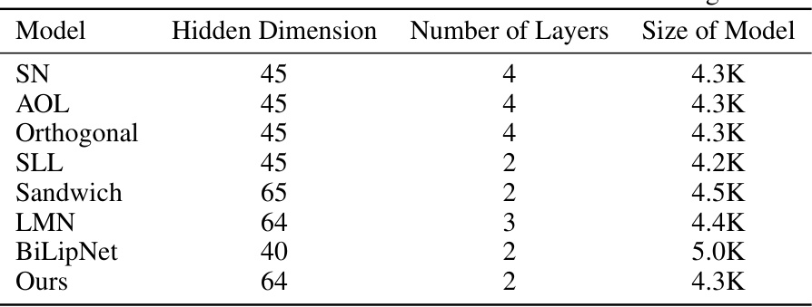
This table compares the tightness of Lipschitz bounds for various bi-Lipschitz models (SN, AOL, Orthogonal, SLL, Sandwich, LMN, BiLipNet) and the proposed model. The models were trained with an upper bound constraint (L) on the Lipschitz constant. The table shows the percentage of how close the actual Lipschitz constant achieved after training is compared to the imposed Lipschitz bound L for each model at different L values (L=2, 5, 10, 50). The results are averaged over five different random seeds.

This table provides details on the architectures used for the uncertainty estimation experiments with the two moons dataset shown in Figure 23. It compares four different models: DUQ, DUQ without regularization, DUQ combined with the proposed Bi-Lipschitz Neural Network (DUQ+BLNN), and Deep Ensembles. For each model, it lists the hidden dimension of the neural network, the number of layers, the output dimension, the centroid size, and the total number of parameters.

This table presents the details of the neural network architectures used in the uncertainty quantification experiments shown in Figure 23 of the paper. It breaks down the specifications for four models: DUQ, DUQ (no regularization), DUQ+BLNN, and Deep Ensembles. For each model, the table lists the hidden dimension, number of layers, output dimension, centroid size, and the total number of parameters.

This table presents the results of an out-of-distribution detection experiment using the FashionMNIST dataset. Two scenarios are compared: FashionMNIST vs. MNIST and FashionMNIST vs. NotMNIST. The performance of two models, DUQ and DUQ+BLNN (Deep Uncertainty Quantification with the proposed Bi-Lipschitz Neural Network), are evaluated using accuracy, binary cross-entropy loss, and AUROC (Area Under the Receiver Operating Characteristic curve) for both MNIST and NotMNIST datasets. The BLNN uses α=0 and β=3.0. The results are averaged over five trials, with standard deviations reported.

This table lists the hyperparameters used for the partially bi-Lipschitz neural network (PBLNN) in the partially monotone settings experiments. It details the hidden dimensions, number of layers, Lipschitz constant, and inverse Lipschitz constant for each dataset (COMPAS, BlogFeedBack, LoanDefaulter, HeartDisease, AutoMPG, CIFAR101). These hyperparameters reflect the architecture’s inductive bias in each experiment.
Full paper#
