Graph Learning for Numeric Planning

↗ OpenReview ↗ NeurIPS Homepage ↗ Chat

TL;DR

#

Key Takeaways

#

Why does it matter?

#

This paper is important because it presents a novel approach to numeric planning, a challenging problem in AI. The data-efficient and interpretable machine learning models offer a significant improvement over existing methods, opening new avenues for research in planning and heuristic learning. Its focus on interpretability and efficiency addresses key limitations of current deep learning approaches, making it particularly relevant to resource-constrained environments. The work also introduces new ranking formulations for improved performance.

Visual Insights

#

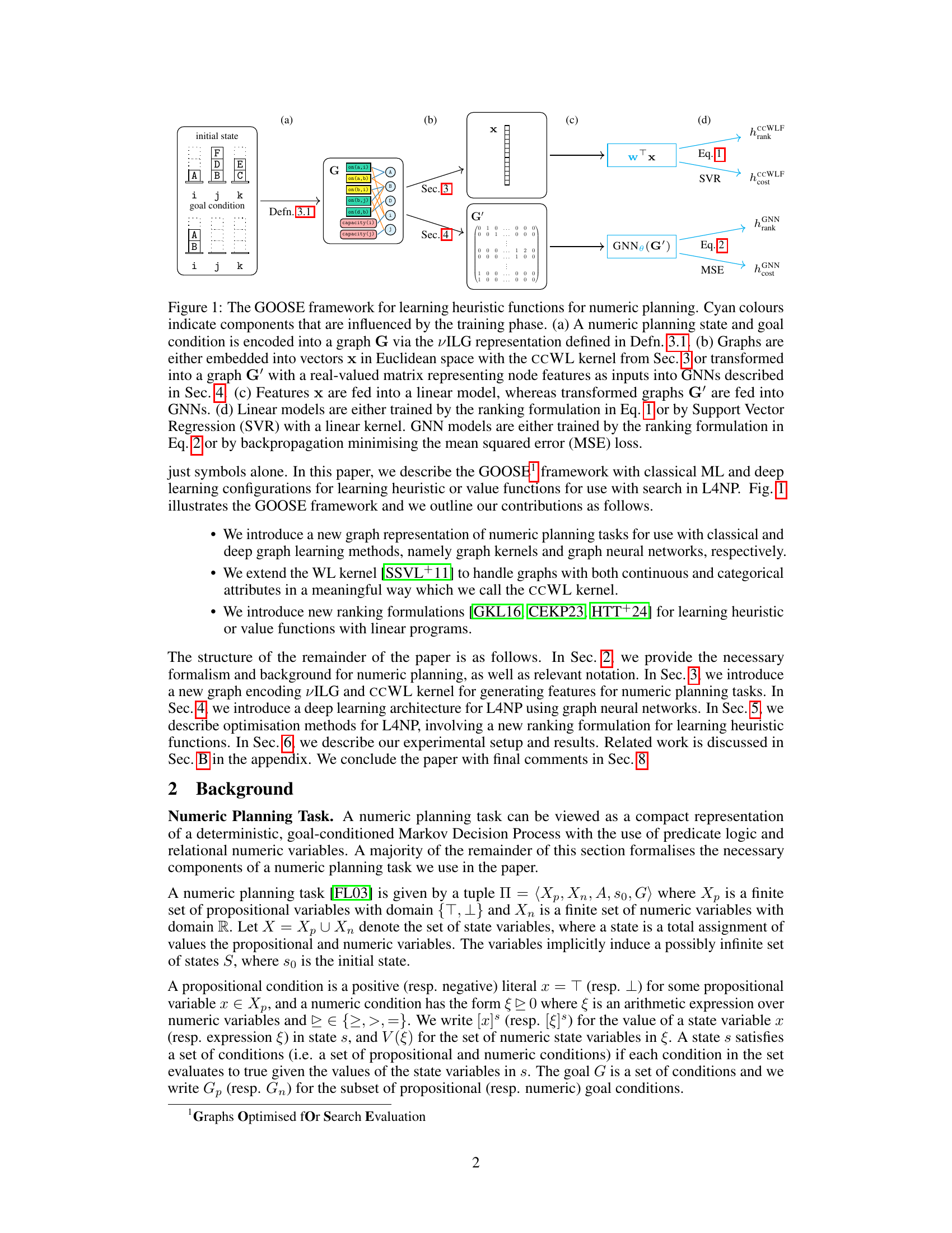
This figure illustrates the GOOSE framework, which is a method for learning heuristic functions for numeric planning. It shows how a numeric planning state and goal are encoded into a graph, which is then processed using either a classical machine learning approach (CCWL kernel and linear model) or a deep learning approach (graph neural network). The resulting heuristic function can then be used in a search algorithm to solve numeric planning problems. The cyan coloring highlights the parts of the system affected by the training phase.

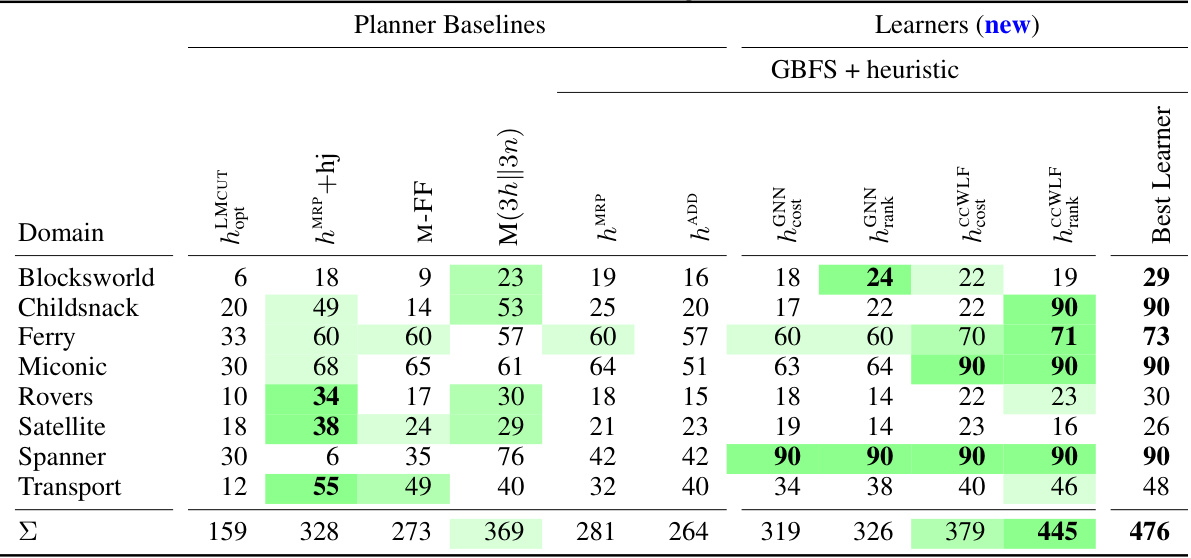
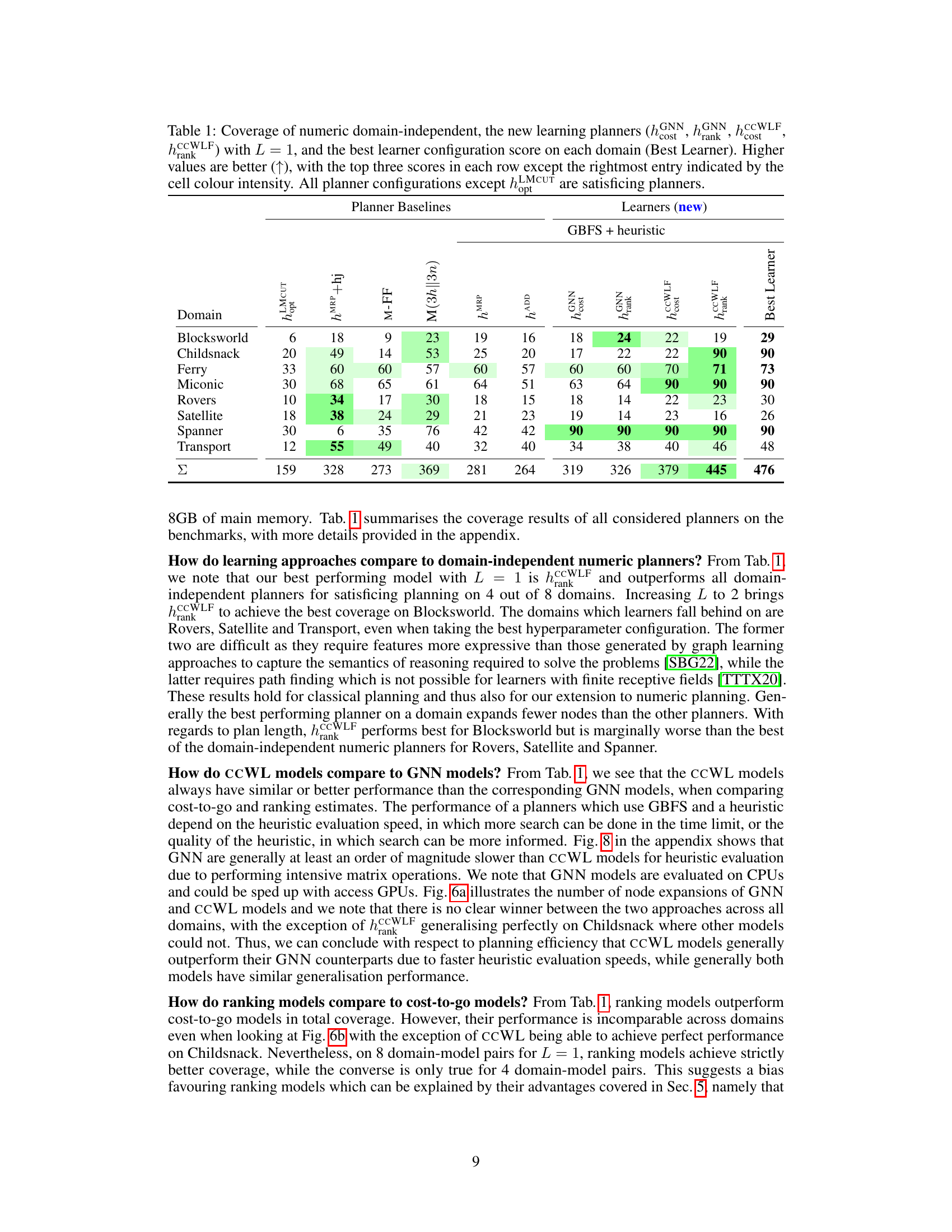
This table presents the performance comparison of various planners on eight numeric planning domains. It shows the number of problems solved (coverage) by different planners, including domain-independent planners and the newly proposed learning-based planners. The table highlights the top three performing planners in each domain, using color coding to indicate performance intensity. It also specifies that the evaluation metric is the number of solved problems, with higher values indicating better performance. Importantly, it notes that all planners except for hMCUT are satisficing (finding any solution) planners, whereas hMCUT is an optimal planner.

In-depth insights

#

Numeric Planning

#

Numeric planning extends classical planning by incorporating numeric variables and arithmetic constraints in state representations and action effects. This introduces significant complexity, as the state space becomes continuous and potentially infinite, making traditional planning techniques computationally expensive or even undecidable. The paper explores machine learning approaches to address this challenge, highlighting the advantages of data-efficient and interpretable models over deep learning methods for learning heuristic functions. Graph-based representations are particularly well-suited for encoding the relational structure of numeric planning problems, allowing for generalization and scalability. The authors introduce a novel graph kernel and ranking-based optimization methods, demonstrating promising results in terms of efficiency and coverage compared to existing numeric planners.

Graph Kernels

#

Graph kernels are functions that measure the similarity between graphs. They are crucial in machine learning for handling graph-structured data, which is common in various fields, including cheminformatics, social networks, and natural language processing. A key advantage of graph kernels is their ability to capture both structural and attribute information of the graphs. Different graph kernel methods exist, each with its strengths and weaknesses. The choice of kernel significantly impacts the performance of machine learning algorithms. Some popular approaches include Weisfeiler-Lehman kernels and random walk kernels. However, designing effective graph kernels can be challenging, especially for large or complex graphs. Furthermore, the computational complexity of kernel computation can limit the scalability of graph kernel methods. Recent research focuses on developing more efficient and expressive graph kernels, as well as exploring their applications in various machine learning tasks. The choice of a suitable kernel often depends on the specific problem and available resources. Therefore, a proper understanding of the kernel’s properties and limitations is vital for building effective graph-based machine learning systems.

GNN Approach

#

The authors explore Graph Neural Networks (GNNs) as an alternative approach for learning heuristic functions in numeric planning. While GNNs are powerful tools for relational data, their application in this context reveals both advantages and limitations. A key advantage is the ability of GNNs to handle graphs of arbitrary sizes, directly addressing the variable-sized nature of numeric planning problems. The network architecture proposed transforms the Numeric Instance Learning Graph (vILG) representation into a format suitable for GNN processing, leveraging both categorical and continuous node features. However, the empirical results indicate that GNNs, while competitive, do not outperform classical machine learning methods based on graph kernels. This suggests that the expressive power of GNNs, while significant, might be less crucial for this specific numeric planning problem compared to the efficiency and generalization capabilities of simpler models. The authors highlight the considerable computational cost associated with training and using GNNs, emphasizing that simpler models achieve better results in terms of coverage and efficiency. This finding underscores the need for careful model selection in L4NP, balancing expressive power with computational constraints and generalization performance. Further investigation is needed to determine if more sophisticated GNN architectures or training methods could improve performance.

Learning Heuristics

#

Learning effective heuristics for planning problems, especially in numeric domains, presents a significant challenge. This involves finding ways to efficiently estimate the cost or difficulty of reaching a goal state from a given state. The use of machine learning techniques offers a promising avenue for automating heuristic generation. Instead of relying on handcrafted heuristics, which are often domain-specific and time-consuming to develop, machine learning models can learn these heuristics from data. The choice of a suitable machine learning model is critical, with considerations given to data efficiency, generalizability, and interpretability. For instance, classical machine learning models might be preferred for their efficiency and interpretability over deep learning models, especially when dealing with limited training data. However, the representation of the problem (e.g., using graphs) significantly impacts the effectiveness of learning. A careful design of the problem representation that captures the relevant structural information is crucial for generating useful heuristic functions. Moreover, the choice of optimization method for training the learning models influences the quality of learned heuristics. For example, methods based on ranking heuristics could offer advantages over those solely focusing on minimizing cost-to-go estimates, especially with regard to generalization capabilities. The success of learning heuristics depends on a careful consideration of all these intertwined factors. Ultimately, the evaluation of learned heuristics should be performed using a broad range of metrics and benchmark planning problems to ensure generalizability and effectiveness beyond training data.

Future of L4NP

#

The future of Learning for Numeric Planning (L4NP) is promising, with several key directions emerging. Improved graph representations are crucial, moving beyond simple encodings to capture richer relational and numerical interactions within planning domains. This includes exploring advanced graph neural networks (GNNs) architectures and more sophisticated graph kernels to handle complex relationships and continuous features. Data efficiency remains a major challenge; methods to learn from smaller datasets, perhaps leveraging transfer learning or meta-learning techniques, are vital. Addressing the scalability issue will require exploring more efficient training and inference techniques, potentially focusing on distributed training or approximate inference. Finally, incorporating domain knowledge more effectively will enhance generalisation capabilities and reduce overfitting. Integrating symbolic reasoning with learned numerical components holds great potential, combining the strengths of both paradigms. Overall, the success of L4NP will depend on tackling these challenges through novel theoretical advancements and innovative application of existing and future machine learning technologies.

More visual insights

#

More on figures

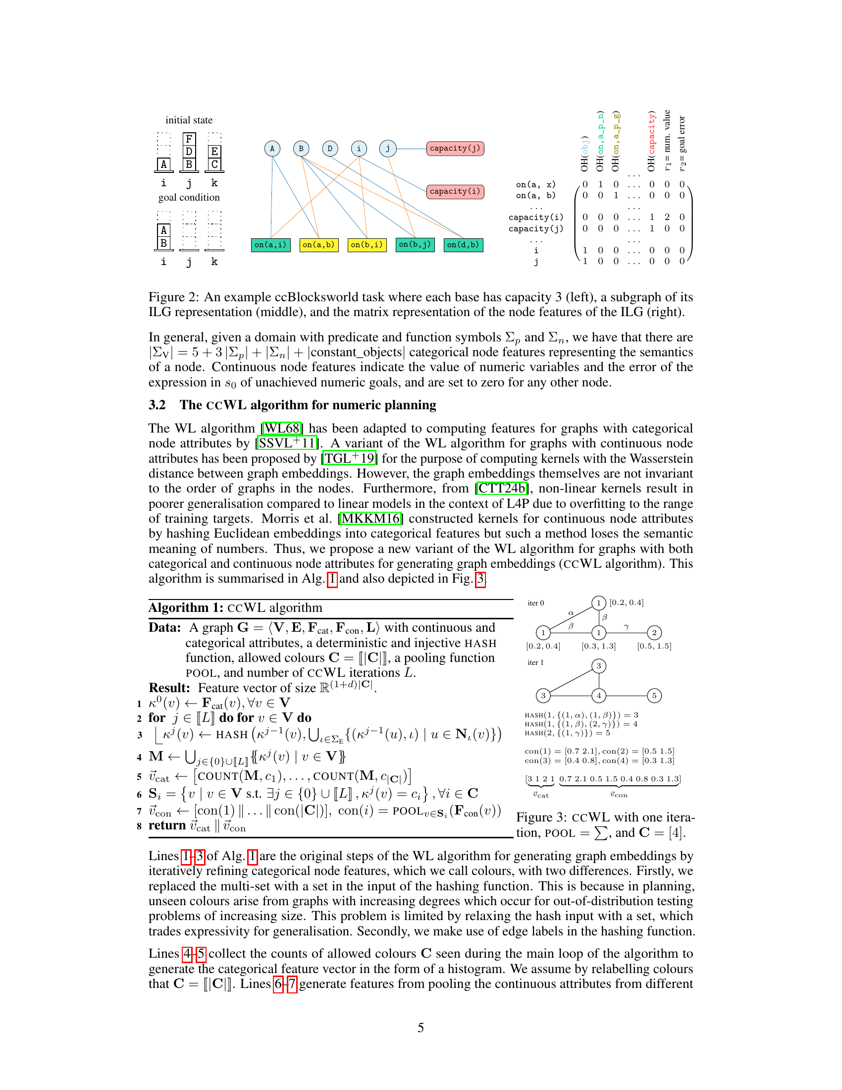
This figure illustrates an example of Capacity Constrained Blocksworld (ccBlocksworld) planning task, showing its representation in three different ways: (left) a visual representation of the initial state and goal condition; (middle) a subgraph of its Numeric Instance Learning Graph (vILG) representation showing the nodes (objects, variables, and goals) and edges representing relationships between them; and (right) a matrix representation of the node features in the vILG, showing both categorical and continuous features used to encode the planning problem.

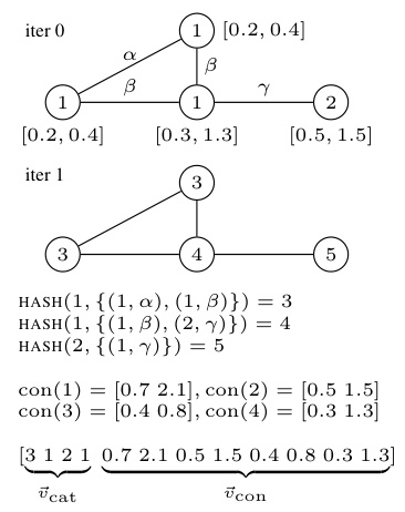
This figure illustrates the GOOSE framework, a machine learning approach for solving numeric planning problems. It shows how a numeric planning state and goal are encoded as a graph (a). This graph is then processed using either a classical method (CCWL kernel, embedding to vector) or a deep learning method (GNN, transformation to graph G’). Finally, the resulting features are used to train linear models or GNNs using ranking formulations or MSE loss (d). The cyan color highlights the components modified during training.

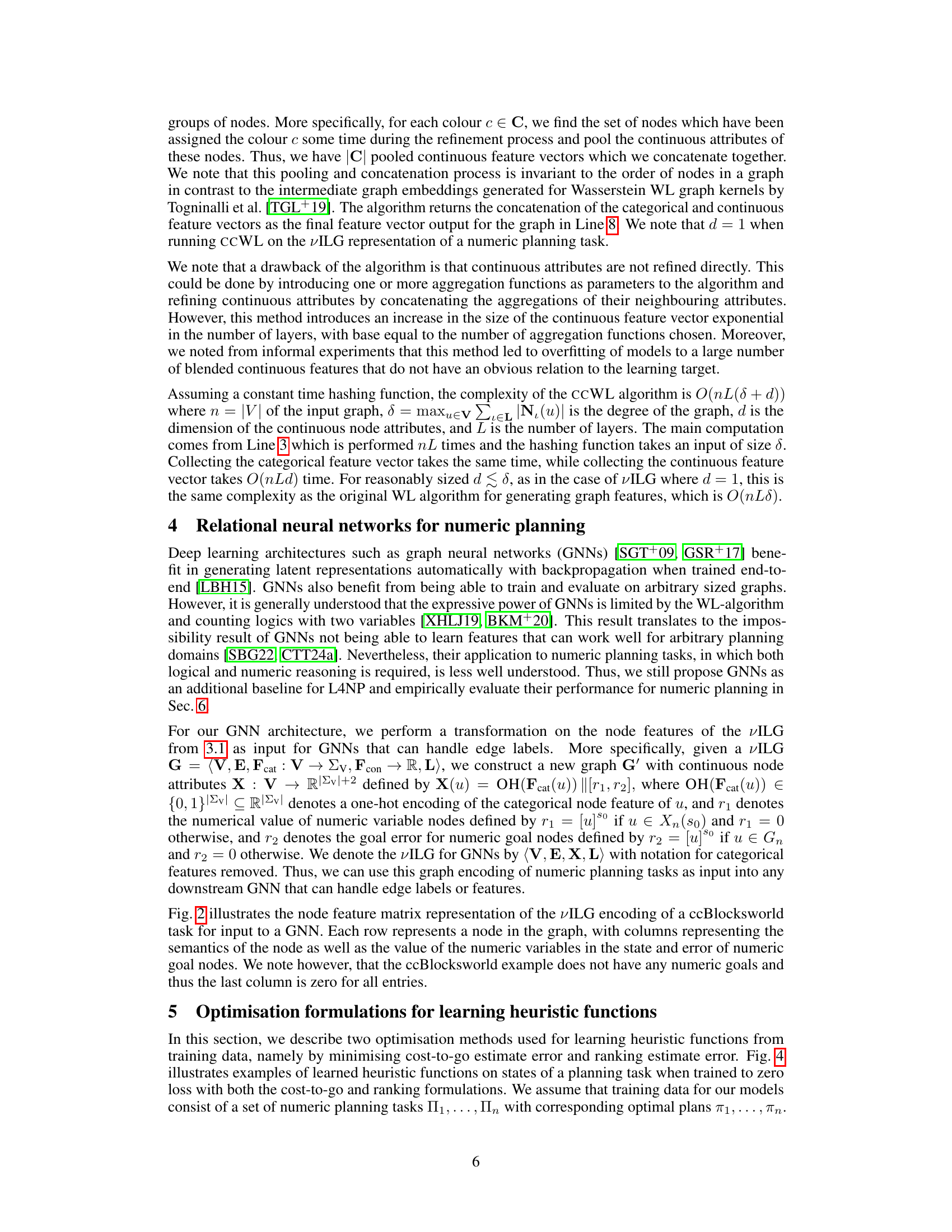
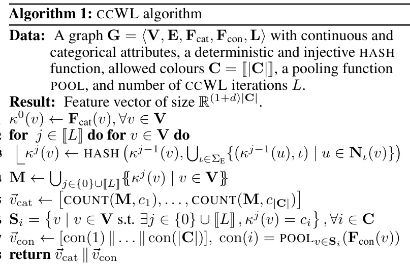
This figure illustrates one iteration of the CCWL algorithm. It shows how categorical and continuous node features are processed. Categorical features (colors) are updated using a hash function that incorporates both the node’s current color and the colors of its neighbors. Continuous features are pooled (summed in this example) for each color group. The resulting combined categorical and continuous features are used to generate the final feature vector for the graph.

This figure shows examples of heuristic functions that achieve zero loss when optimizing either for cost-to-go or ranking. The left side shows a cost-to-go heuristic, which can achieve zero loss on the optimal plan path, but may not generalize well to other states. The right side demonstrates a ranking heuristic, which doesn’t need perfect cost-to-go values but only needs to maintain correct rankings between states. The figure highlights that the Greedy Best First Search (GBFS) algorithm is significantly more efficient for ranking heuristics than cost-to-go heuristics.

This figure presents a comparative analysis of the number of objects across different domains used in the training and testing phases of the experiments. The left panel displays bar charts showing the number of objects (on a logarithmic scale) in the training and testing datasets for each of eight domains: Blocksworld, Childsnack, Ferry, Miconic, Rovers, Satellite, Spanner, and Transport. The right panel uses box plots to illustrate the distribution of training data generation times (also on a logarithmic scale) for each domain, providing insight into the computational effort required for data preparation in each case. This helps to understand the resources needed and potential differences in training times for each domain.

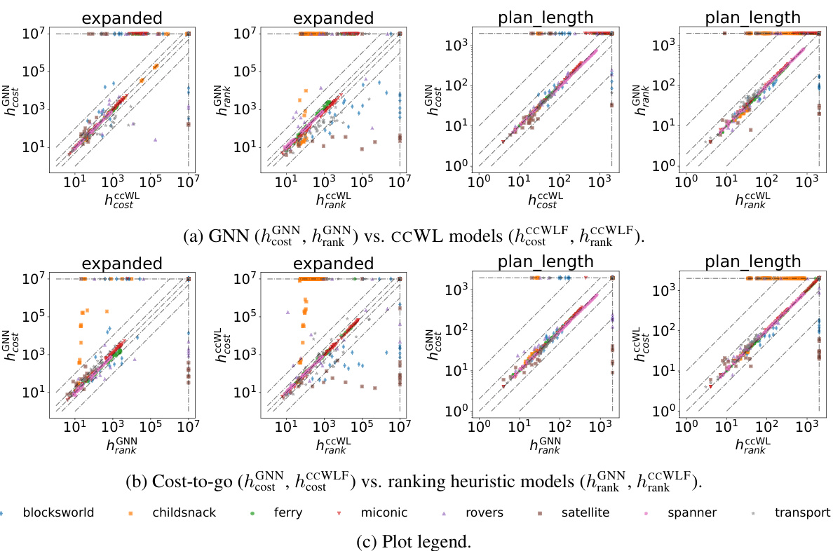
This figure compares the performance of different models in terms of the number of nodes expanded and the plan length generated. Each plot shows a comparison between two model types across eight domains. The points in the plot represent the performance metrics (x,y) for each domain; points in the top-left quadrant indicate better performance for the model on the x-axis, while those in the bottom-right quadrant suggest better performance for the model on the y-axis. The plots help to visually assess the relative strengths and weaknesses of the different models.

This figure shows an example of a Capacity Constrained Blocksworld planning task. The left side depicts the initial state of the problem: blocks stacked on three bases, each with a capacity of 3 blocks. The middle shows a subgraph of the Numeric Instance Learning Graph (vILG) representation of this task. The nodes in the graph represent objects, propositional variables, numeric variables, and goal conditions, while edges connect these nodes based on their relationships. The right side displays the node feature matrix of the vILG. This matrix encodes the categorical and continuous node features (such as object type, propositional/numeric variable values, etc.) as input for later machine learning methods.

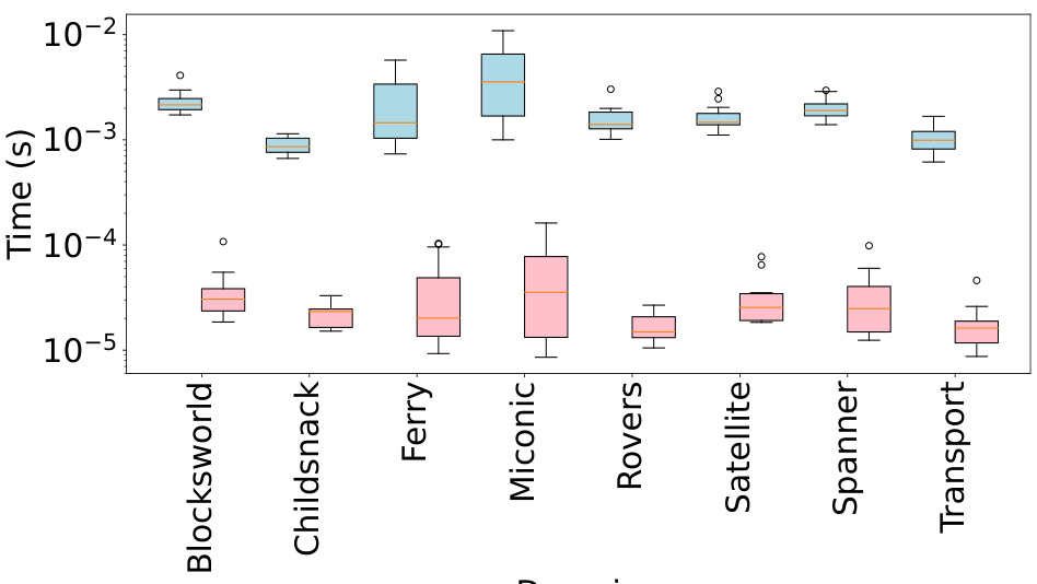
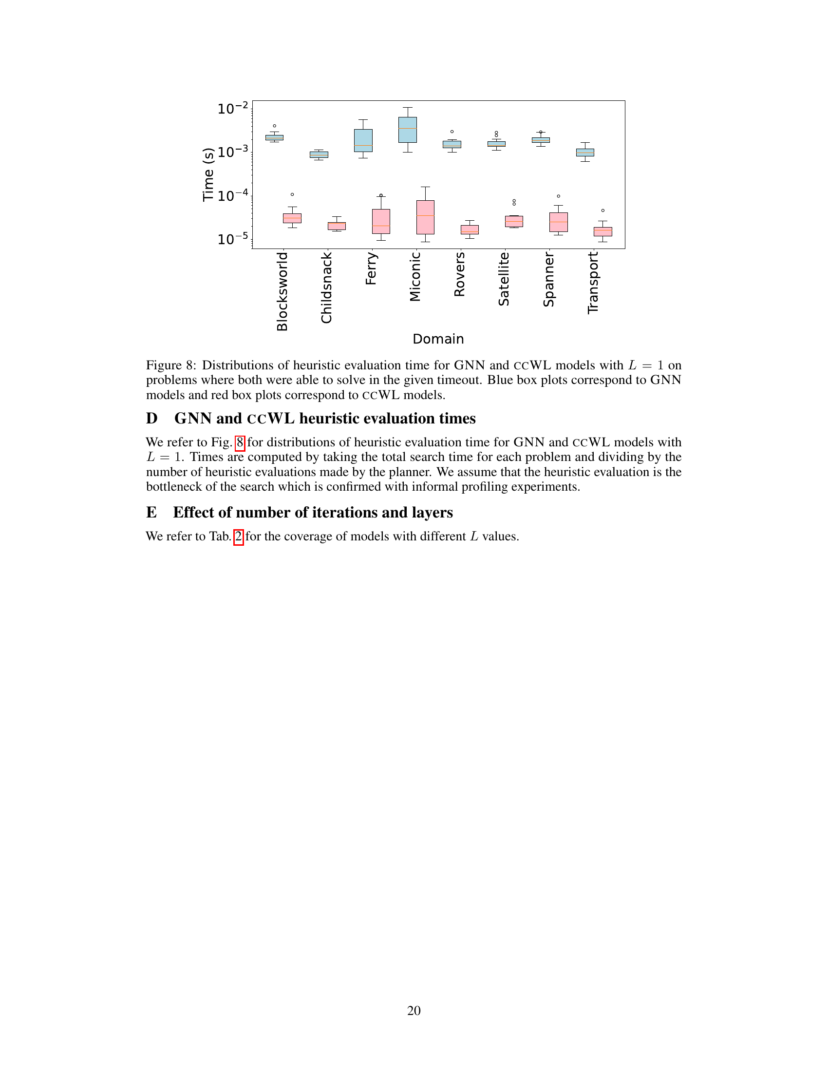
This figure shows the distribution of heuristic evaluation times for Graph Neural Networks (GNNs) and the Color-Coded Weisfeiler-Lehman (CCWL) algorithm. The box plots display the median, quartiles, and outliers for each model across various planning domains. Blue boxes represent GNNs, while red boxes represent CCWL. The results illustrate the relative computational efficiency of each method for heuristic computation within the context of numeric planning.

More on tables

This table shows the performance of CCWL and GNN models with different numbers of iterations (for CCWL) and layers (for GNNs). It presents the coverage (percentage of problems solved) and median number of expansions for each model across eight planning domains. Higher coverage is better, while a lower median number of expansions indicates greater efficiency. The best performing model for each metric (coverage and expansions) in each domain is highlighted.

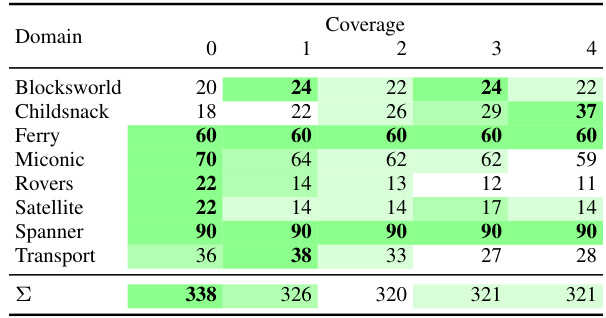
This table presents the performance of CCWL and GNN models with varying numbers of iterations (for CCWL) and layers (for GNN). It shows the coverage (percentage of problems solved) and median number of node expansions for each model across different planning domains. Higher coverage indicates better performance, while lower expansions represent greater efficiency.

This table shows the performance of CCWL and GNN models with different numbers of iterations (for CCWL) and layers (for GNN). It presents the coverage (number of problems solved) and median number of node expansions for each model across eight planning domains. The best performing model (highest coverage/lowest expansions) for each domain and metric is highlighted.

This table shows the performance of different models (CCWL and GNN) with varying numbers of iterations/layers. It presents the coverage (number of problems solved) and median number of node expansions for each model and domain. The best performing model for each domain in terms of coverage and expansion is highlighted.

Full paper

#