↗ OpenReview ↗ NeurIPS Homepage ↗ Chat
TL;DR#
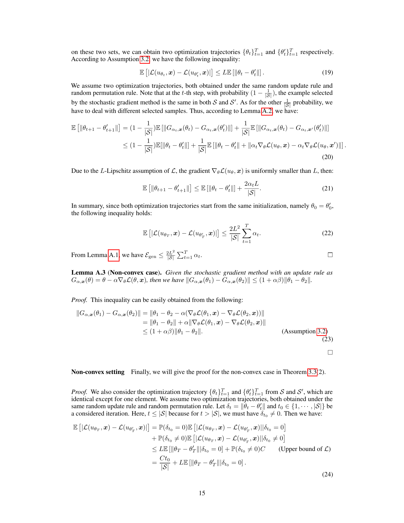
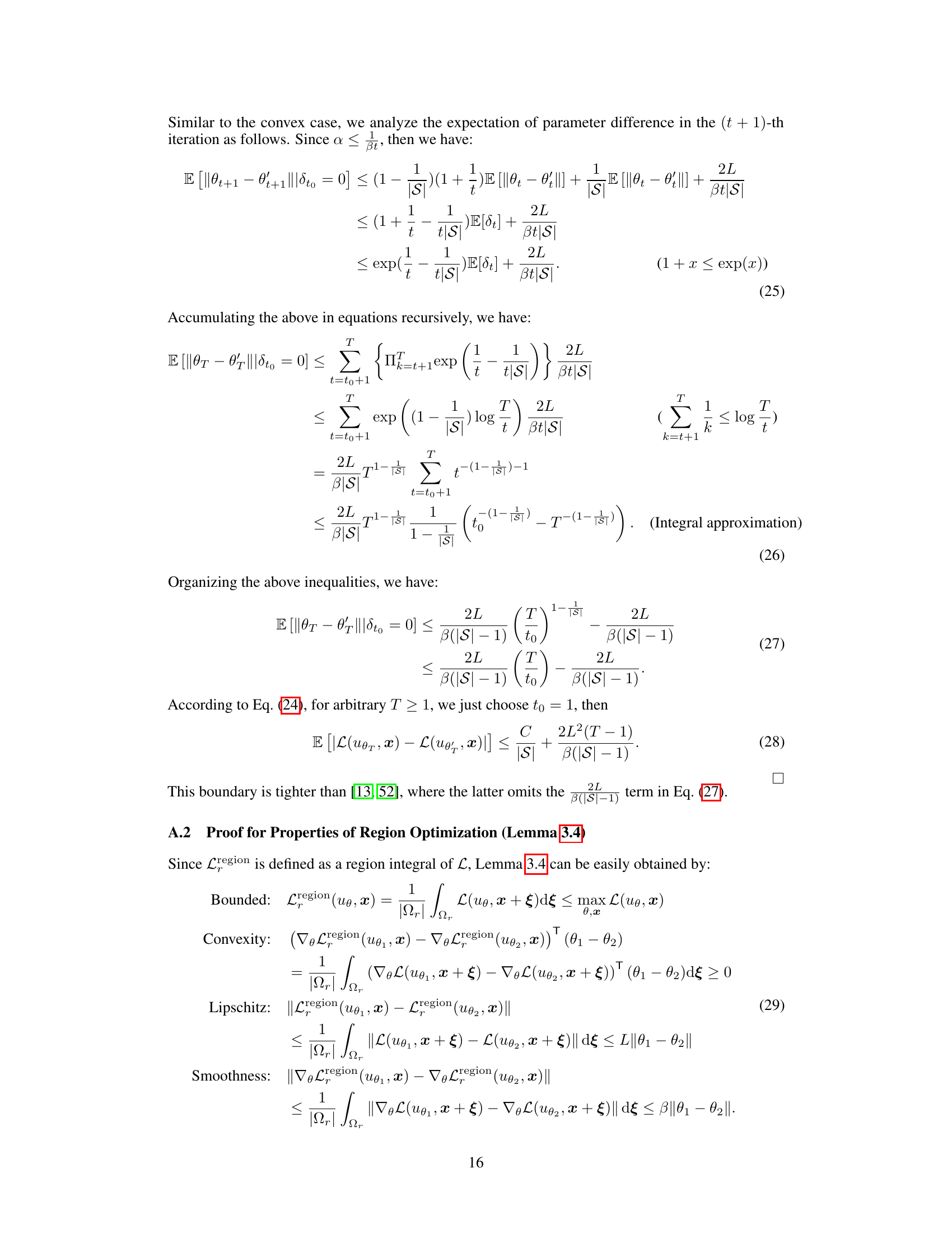
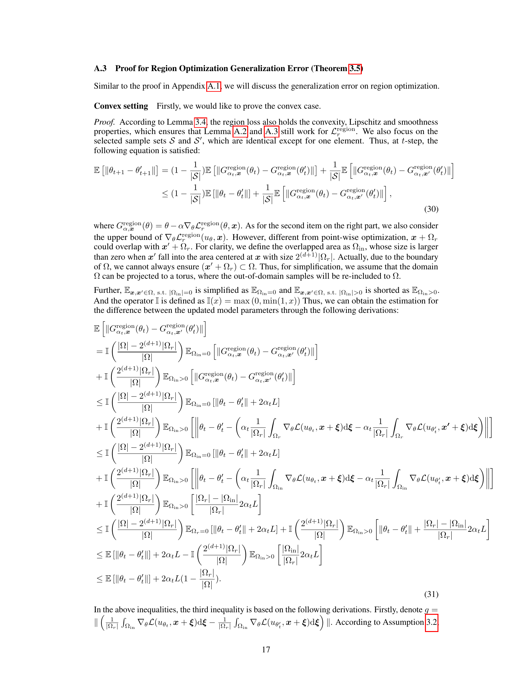
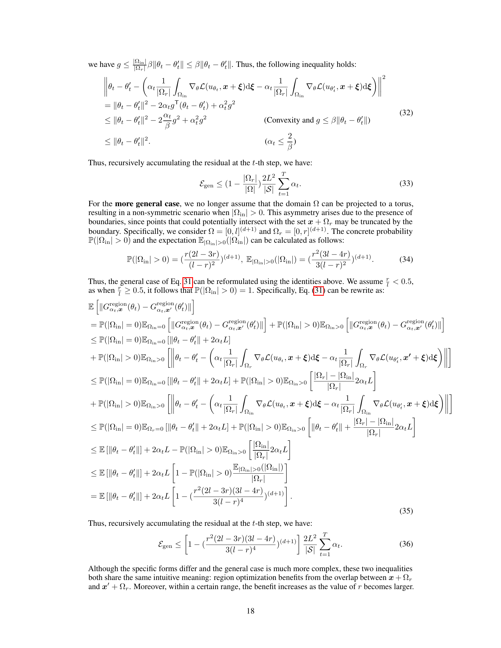
Physics-Informed Neural Networks (PINNs) effectively solve partial differential equations (PDEs), but their conventional point-wise optimization can result in inaccurate solutions and high generalization error, particularly for high-order PDEs. This is because the discrete sampling of points fails to capture the continuous nature of PDEs.
To address this, RoPINN introduces a novel region optimization paradigm. By extending the optimization process from individual points to their continuous neighboring regions, RoPINN leverages a simple Monte Carlo sampling to improve accuracy and generalizability, effectively calibrating the sampling process to ensure both optimization and generalization. Extensive experimental results on various PDEs demonstrate RoPINN’s efficacy and broad applicability across different PINN architectures, improving the state-of-the-art performance without any increase in computational overhead.
Key Takeaways#
Why does it matter?#
This paper is crucial for researchers working with physics-informed neural networks (PINNs). It introduces a novel training paradigm that significantly improves PINN accuracy and generalizability, addressing a long-standing limitation. The proposed RoPINN method offers a practical and efficient solution, opening new avenues for tackling complex partial differential equations (PDEs) across diverse scientific domains. The theoretical analysis provides a solid foundation for future work, while the consistent improvements demonstrated across various benchmark PDEs and PINN architectures highlight its broad applicability.
Visual Insights#

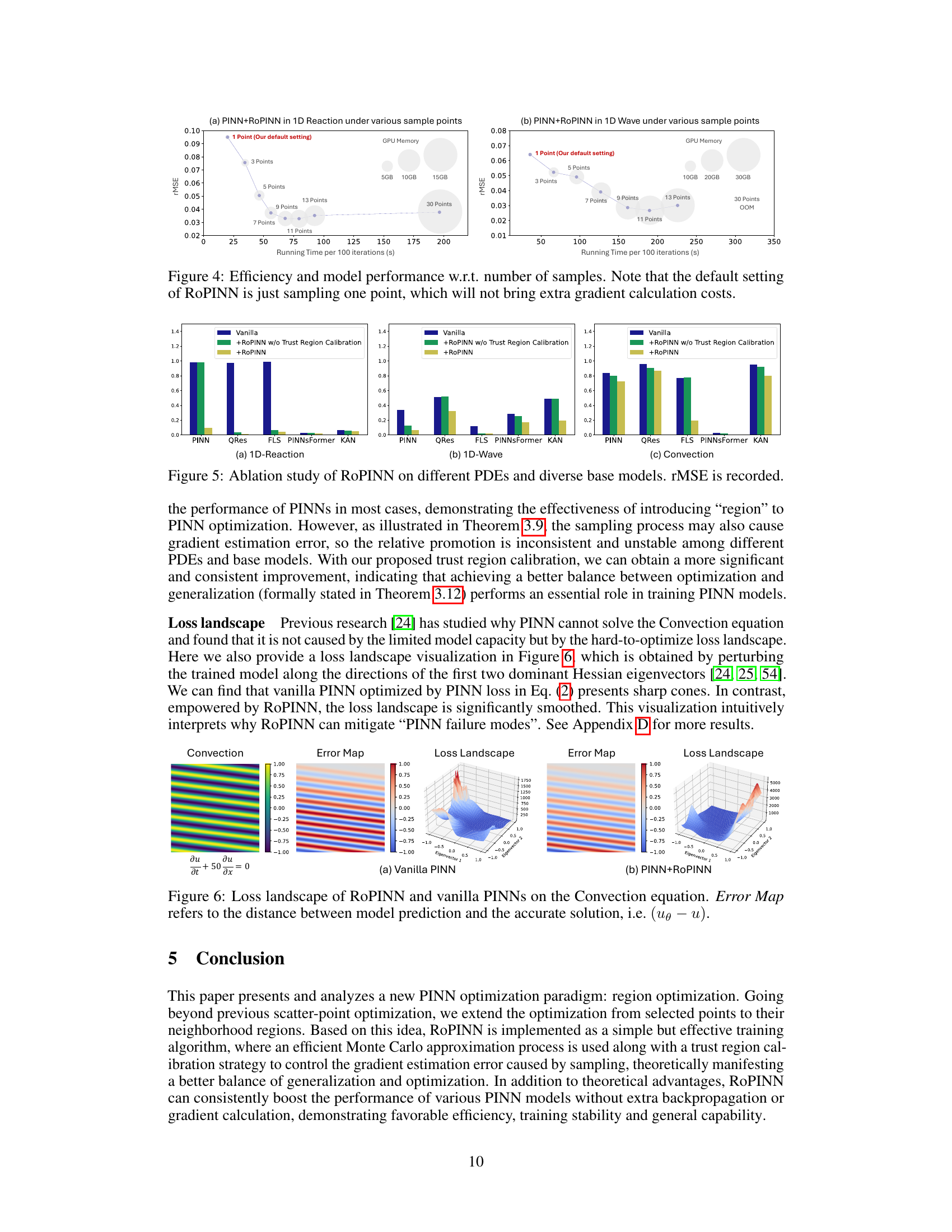
This figure shows the results of experiments on the 1D-Reaction benchmark using canonical PINN. Different initial trust region sizes (r) were tested, and the plots show how the trust region size, training loss, and test rMSE (root mean squared error) evolve over training iterations. The moving average of the trust region size is displayed, with the standard deviation shaded. The plots illustrate how RoPINN adjusts the trust region size and impacts the model’s convergence and generalization.

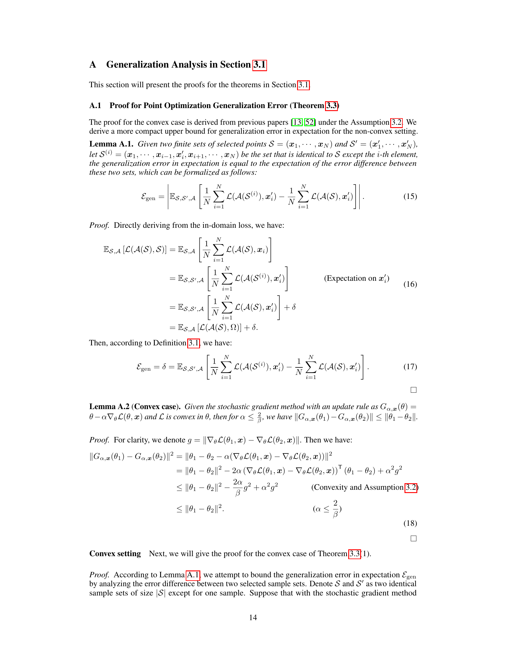
This table compares the performance of RoPINN against gPINN and vPINN across various base models and benchmark PDEs. It shows the loss (loss function), mean absolute error (MAE), and root mean squared error (RMSE) for each method, highlighting improvements over the standard PINN. The PINNacle results display the percentage of tasks where RoPINN improved upon the vanilla PINN. ‘Promotion’ indicates the percentage increase in performance achieved by RoPINN over the standard PINN.
In-depth insights#
ROPINN: Core Idea#
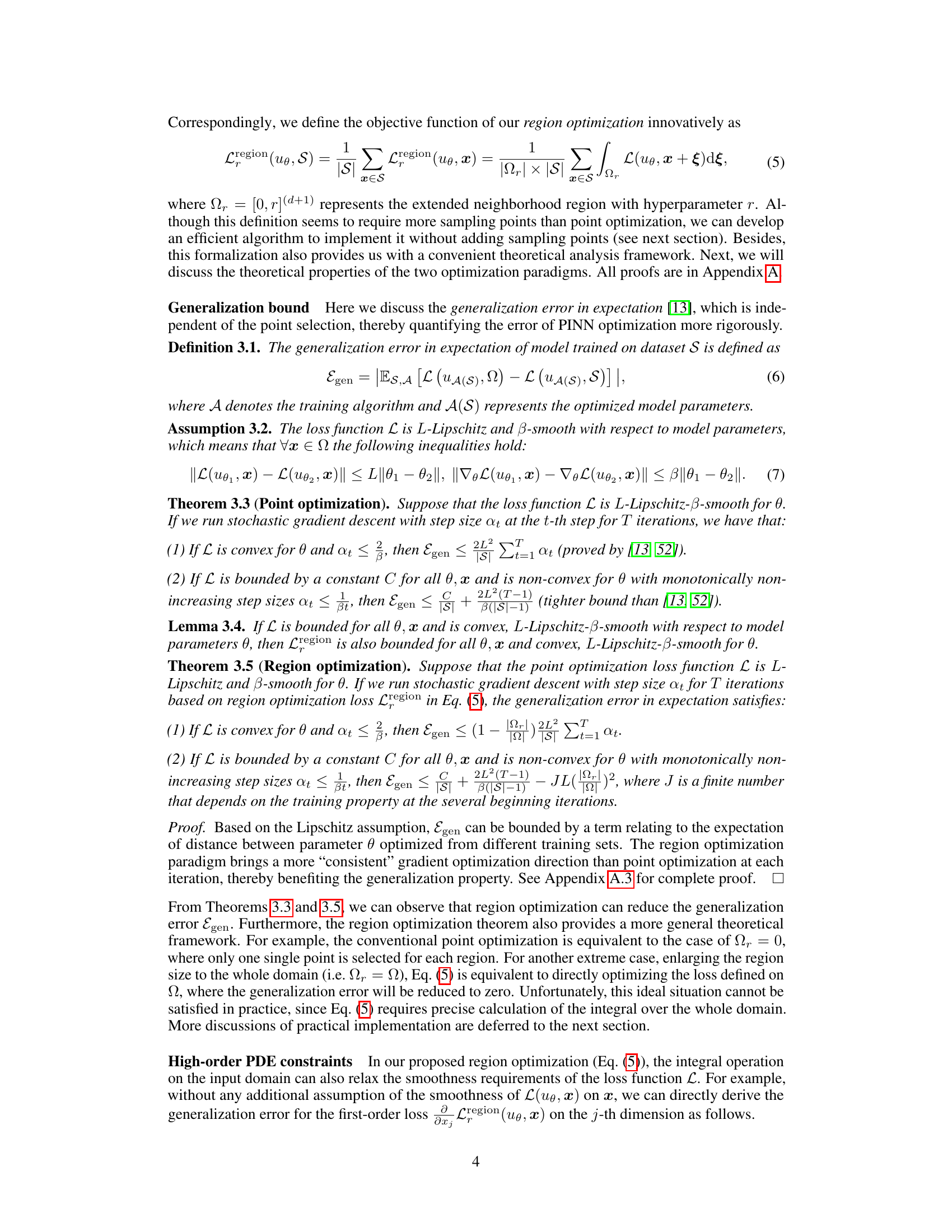
ROPINN’s core idea centers on region optimization for Physics-Informed Neural Networks (PINNs). Unlike traditional PINNs which optimize on scattered points, potentially missing crucial information between these points, ROPINNs extend the optimization to continuous neighborhood regions. This addresses the inherent limitation of point-based optimization by considering the continuous nature of PDEs, leading to improved generalization and handling of high-order constraints. The practical implementation uses Monte Carlo sampling within these regions, and a trust region calibration strategy to control estimation error, balancing the trade-off between optimization and generalization. The method’s strength lies in its ability to enhance PINN performance for diverse PDEs without requiring extra backpropagation or gradient calculations, making it a more efficient and effective training paradigm for solving partial differential equations.
Regional Optimization#
The concept of “Regional Optimization” in the context of Physics-Informed Neural Networks (PINNs) offers a compelling alternative to traditional point-wise optimization methods. Instead of solely focusing on individual points for loss calculation, regional optimization expands the optimization process to encompass entire neighborhoods surrounding each point. This approach fundamentally addresses the inherent limitation of PINNs, which are typically trained on discrete samples despite solving continuous PDEs. By considering the continuous behavior within regions, regional optimization can potentially mitigate generalization error, especially when dealing with high-order PDE constraints where isolated point evaluations might be insufficient. The core idea lies in smoothing the loss landscape through aggregation, making the optimization process more stable and less susceptible to noise arising from sparse data. This method also has the potential to naturally incorporate high-order derivative information without explicit calculation, thereby improving accuracy and stability. However, the effectiveness of regional optimization hinges on carefully balancing the size of the regions and the associated computational cost. Overly large regions can lead to increased computational burden and may smooth out critical information, reducing the training accuracy. Therefore, a well-defined method for selecting and adapting region size, such as the trust region calibration proposed, is crucial for practical implementation.
Trust Region Tuning#
Trust region methods are iterative algorithms used in optimization to find a local minimum of an objective function. In the context of physics-informed neural networks (PINNs), a trust region approach is particularly valuable because PINN loss functions often exhibit complex behavior. A trust region mechanism dynamically adjusts the size of the region around the current parameter values where the model’s approximation of the loss is considered reliable. This adaptive behavior helps to balance the exploration-exploitation trade-off: too large a region risks unstable updates, while a region that’s too small could hinder convergence speed. The tuning process typically involves monitoring the model’s performance and gradient information within the trust region; this information informs whether to expand or contract the region. Effective trust region tuning is crucial for efficient and reliable PINN training. It’s critical that the trust region is neither too large (leading to potentially inaccurate gradient estimates and unstable updates), nor too small (resulting in slow convergence). The effectiveness of a trust region method for PINNs is dependent on several factors, including the choice of the trust region update strategy and the method for estimating the loss and gradient within the region. Monte Carlo sampling is one way to estimate the loss in the trust region, offering a flexible strategy that is simple to implement, but the accuracy of the estimate is important to consider.
High-Order PDEs#
High-order partial differential equations (PDEs) pose significant challenges in numerical computation due to their inherent complexity and the increased computational cost associated with approximating higher-order derivatives. Standard numerical methods often struggle with accuracy and stability when dealing with these equations, especially in the presence of discontinuities or complex geometries. Physics-informed neural networks (PINNs) offer a promising alternative approach. However, even PINNs face difficulties when directly enforcing high-order PDE constraints because high-order gradients can be unstable and time-consuming to compute. This limitation is further compounded by the fact that PINNs typically rely on point-wise optimization, which can lead to inaccurate solutions in the whole domain. Region optimization, as proposed by RoPINN, presents a more robust paradigm by extending the optimization process from isolated points to their continuous neighborhood regions. This approach theoretically reduces the generalization error, which is particularly beneficial for capturing hidden high-order constraints inherent in many high-order PDEs. Furthermore, Monte Carlo sampling methods, as used in RoPINN, offer a practical approach to implement region optimization efficiently, without requiring additional gradient calculations or substantial computational overhead. The trust region calibration strategy in RoPINN finely balances optimization and generalization, ensuring reliable convergence and high accuracy even when dealing with complex, high-order PDEs.
Limitations & Future#
A research paper’s “Limitations & Future” section would critically examine the study’s shortcomings. Limitations might include the scope of the dataset (e.g., limited geographical representation, specific time period), the methodology’s assumptions (e.g., linearity, independence), or the generalizability of findings to different contexts. The discussion should acknowledge any potential biases or confounding variables that could affect the results’ interpretation. Future work could involve expanding the dataset to improve representativeness, refining the methodology to address identified limitations (e.g., using more robust statistical techniques), or exploring how the findings might generalize to other populations or settings. It might also suggest new research questions or areas for investigation arising from this study’s results. A strong “Limitations & Future” section demonstrates intellectual honesty, and provides a roadmap for subsequent research to address the gaps and advance knowledge.
More visual insights#
More on figures

This figure shows the results of training a canonical PINN on the 1D-Reaction problem using different initial region sizes for the RoPINN algorithm. It demonstrates how RoPINN adjusts the trust region size over training iterations to find a balance between training stability and generalization. The plots show the trust region size, training loss, and test rMSE for various initial region sizes. The shadow around the region size curves indicates the temporal standard deviation, providing insight into the dynamic adjustments made by RoPINN.

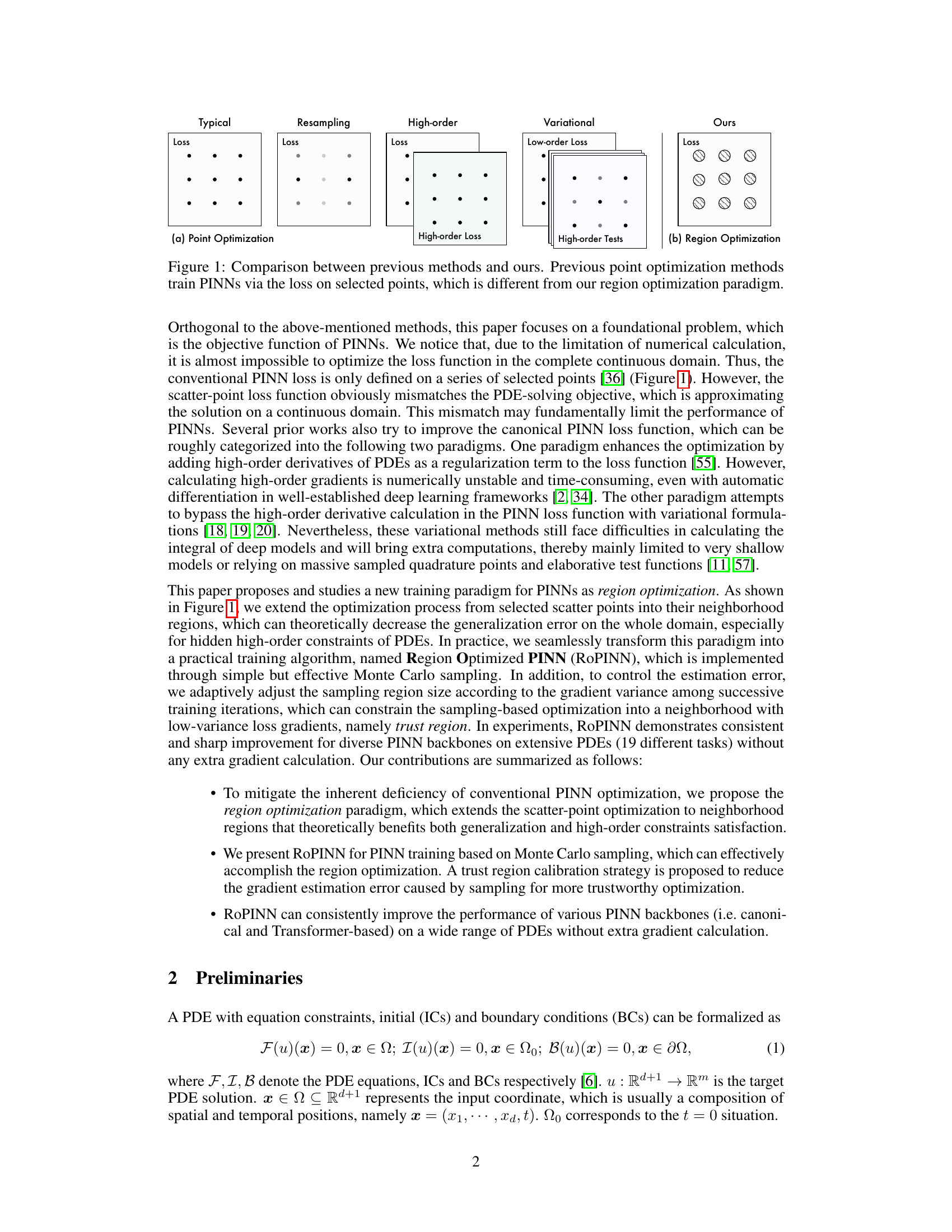
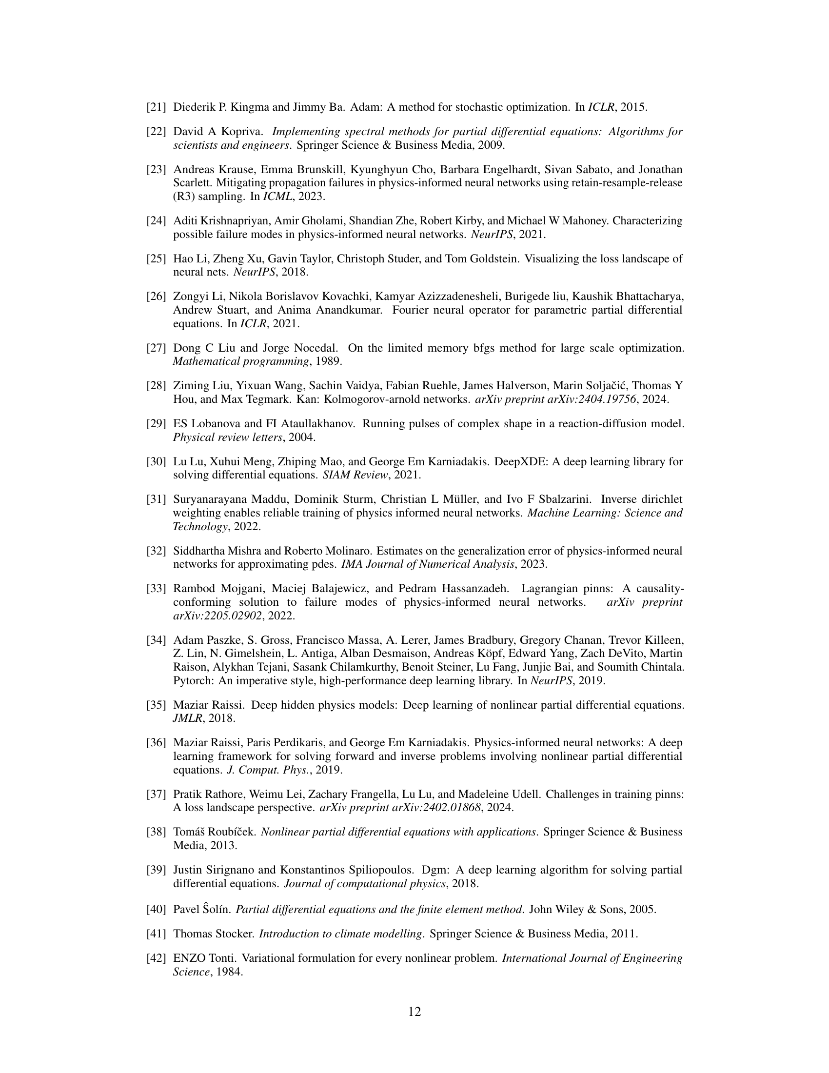
This figure compares point optimization methods with the proposed region optimization method. Point optimization methods use the loss function evaluated at a finite set of scattered points to train the physics-informed neural network (PINN). The authors propose region optimization, which extends the optimization process from these individual points to their surrounding continuous regions. This is illustrated visually by showing how the optimization process differs—the loss is calculated over a set of points in point optimization, but it’s calculated over a region surrounding each point in region optimization.

This figure compares different PINN training methods. Point optimization methods, shown on the left, focus on minimizing loss at specific, selected points within the problem domain. In contrast, the authors’ proposed region optimization method, shown on the right, expands the optimization to encompass the continuous neighborhood around each point, leading to a more robust and generalized solution. This expansion aims to address the inherent limitations of using only scattered points for training models intended to solve continuous problems.

This figure compares different training methods for Physics-Informed Neural Networks (PINNs). Previous methods, shown on the left, optimize the PINN loss function only at a small number of discrete, selected points within the solution domain. In contrast, the authors’ proposed method (ROPINN), shown on the right, optimizes the loss function across entire regions surrounding each selected point, rather than just the points themselves. This regional optimization approach is intended to improve the accuracy and generalization ability of the PINN model.

This figure compares different PINN training methods. The left side shows typical point optimization methods, which focus on calculating the loss at specific, selected points. The right side shows the proposed region optimization method, which instead calculates the loss over continuous regions surrounding the selected points. This extension from points to regions is the core difference and is intended to improve the accuracy and generalization of the PINN model by better representing the continuous nature of PDEs.

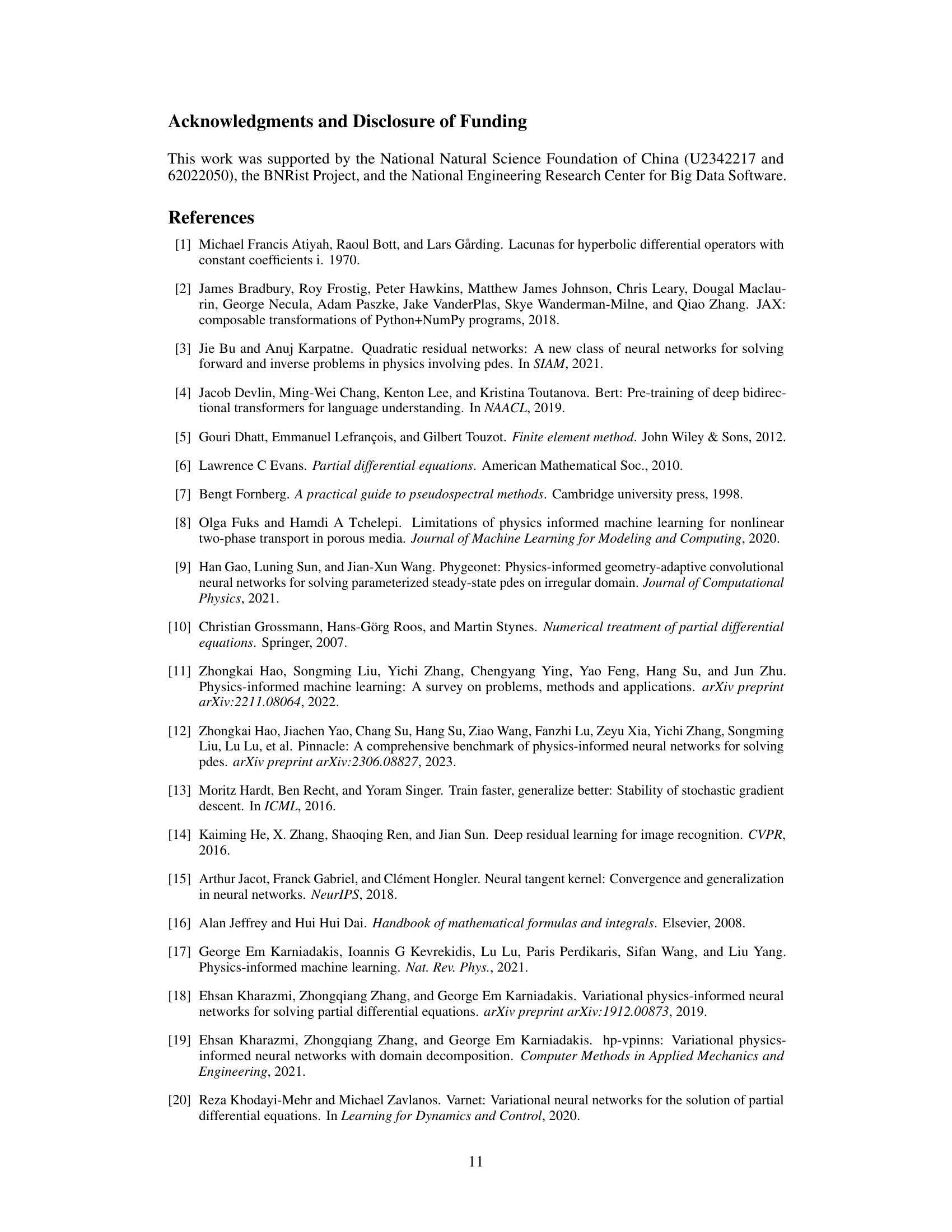
The figure shows the effect of the hyperparameter To (number of past iterations retained to estimate the trust region) on the performance of RoPINN. Four subfigures illustrate the results for different model-benchmark combinations (1D-Reaction PINN, 1D-Wave PINN, Convection PINN, and Convection PINNsFormer). It demonstrates that RoPINN consistently outperforms vanilla PINN across various To values but suggests a potential optimal range for To that balances training stability and generalization.
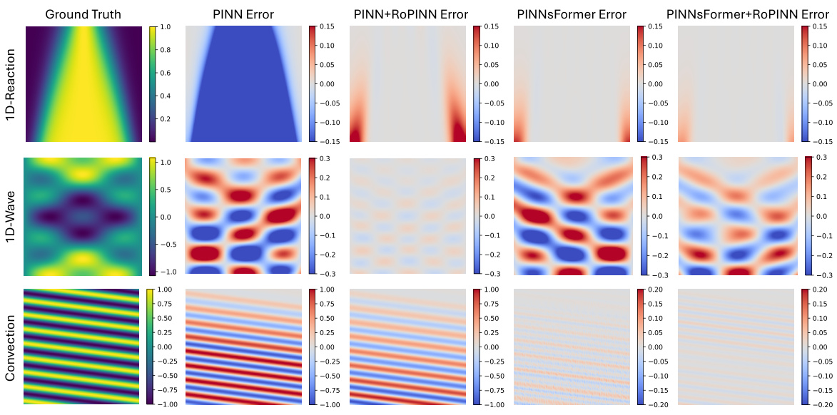
This figure compares different optimization methods for Physics-Informed Neural Networks (PINNs). The typical approach, point optimization, trains the PINN by minimizing the loss function calculated at only a few selected points. This is contrasted with the novel region optimization method proposed in the paper, which expands the optimization process from isolated points to their surrounding continuous neighborhood regions. This visual helps illustrate the key difference between the established methodology and the author’s proposed improvement.
More on tables

This table compares the performance of RoPINN against gPINN and vPINN across various PINN base models (PINN, QRes, FLS, PINNsFormer, KAN) on several benchmarks (1D-Reaction, 1D-Wave, Convection, PINNacle). It shows the loss, rMAE, rMSE values, and the percentage improvement of RoPINN over the standard PINN for each task. The PINNacle results are presented as the proportion of improved tasks. The table highlights the superior performance of RoPINN in most cases.
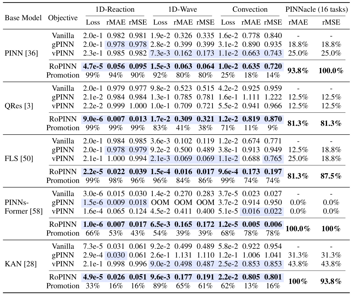
This table compares the performance of RoPINN against gPINN and vPINN across various PINN base models on several benchmark PDEs. It presents loss values (Loss), relative mean absolute error (rMAE), and relative root mean squared error (rMSE) for each model and benchmark. The ‘PINNacle’ section shows the percentage of tasks where RoPINN outperformed the vanilla PINN. The ‘Promotion’ row indicates the percentage improvement achieved by RoPINN compared to the vanilla version. The table highlights the superior and consistent performance of RoPINN.
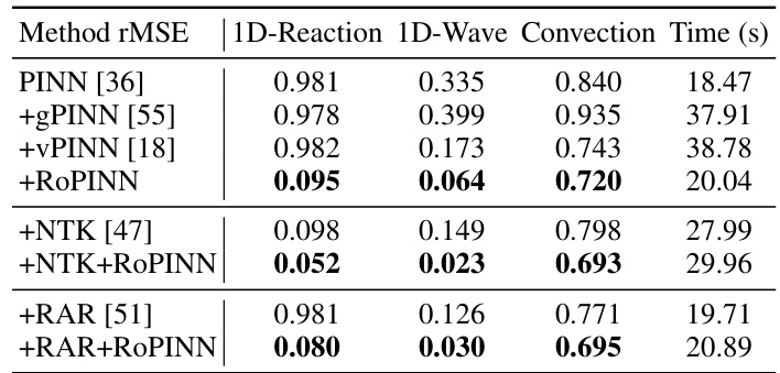
This table compares the performance of RoPINN against two other objective functions (gPINN and vPINN) across various base models for solving different PDEs. The metrics used are training loss, rMAE (relative mean absolute error), and rMSE (relative root mean squared error). The PINNacle benchmark’s results are presented as the percentage of tasks where RoPINN improved upon the vanilla PINN. Blue highlights values exceeding the vanilla PINN’s performance, and bold highlights the best-performing method. The ‘Promotion’ column indicates the performance improvement achieved by RoPINN over the vanilla PINN.

This table compares the performance of RoPINN against two other objective functions (gPINN and vPINN) across various base models for several PDE benchmark problems. It shows loss values (Loss), relative mean absolute error (rMAE), and relative root mean squared error (rMSE) for each model and benchmark. PINNacle results are shown as the percentage of improved tasks. Blue highlighting indicates when RoPINN outperforms the standard PINN, and bold values are the best results. The ‘Promotion’ column indicates the improvement in performance achieved by RoPINN relative to the standard PINN.
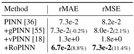
This table compares the performance of RoPINN against two other objective functions (gPINN and vPINN) across various base models (PINN, QRes, FLS, PINNs-Former, KAN) and benchmarks (1D-Reaction, 1D-Wave, Convection, PINNacle). It presents loss, rMAE (relative mean absolute error), and rMSE (relative mean squared error) for each method. The PINNacle results show the percentage of tasks improved by RoPINN compared to the vanilla PINN. Blue highlights indicate when ROPINN outperforms the standard PINN baseline, and bold indicates the best results overall. The table also shows the performance improvement achieved by ROPINN relative to each vanilla PINN.

This table compares the performance of RoPINN against two other objective functions, gPINN and vPINN, across various base models. It shows the loss, rMAE (relative mean absolute error), and rMSE (relative mean squared error) for several PDE benchmarks (1D-Reaction, 1D-Wave, Convection) and the proportion of improved tasks on the PINNacle benchmark. Blue highlights indicate performance superior to the vanilla PINN, while bold indicates the best performance overall.

This table compares the performance of RoPINN against two other objective functions (gPINN and vPINN) across various base PINN models. It shows the loss, rMAE (relative mean absolute error), and rMSE (relative mean squared error) for different PDE benchmarks (1D-Reaction, 1D-Wave, Convection) and the proportion of improved tasks for PINNacle, a more comprehensive benchmark. Blue highlights indicate where RoPINN outperforms the vanilla PINN, and bold indicates the best result. The ‘Promotion’ column shows the percentage improvement achieved by RoPINN over the baseline PINN model.
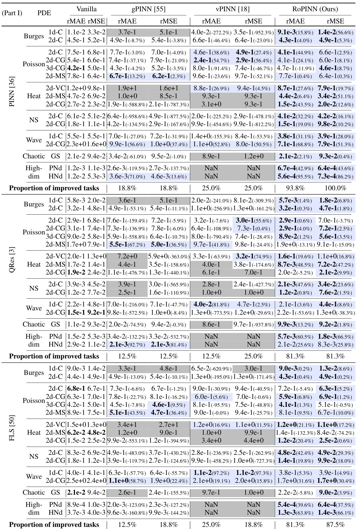
This table compares the performance of RoPINN against gPINN and vPINN across various base models (PINN, QRes, FLS, PINNsFormer, KAN) on multiple PDE benchmark datasets (1D-Reaction, 1D-Wave, Convection, and PINNacle). It shows loss (Loss), relative mean absolute error (rMAE), and relative root mean squared error (rMSE) values. The PINNacle results indicate the percentage of tasks where RoPINN improved performance. Blue highlights values exceeding those of the vanilla PINN, and boldface highlights the best result.
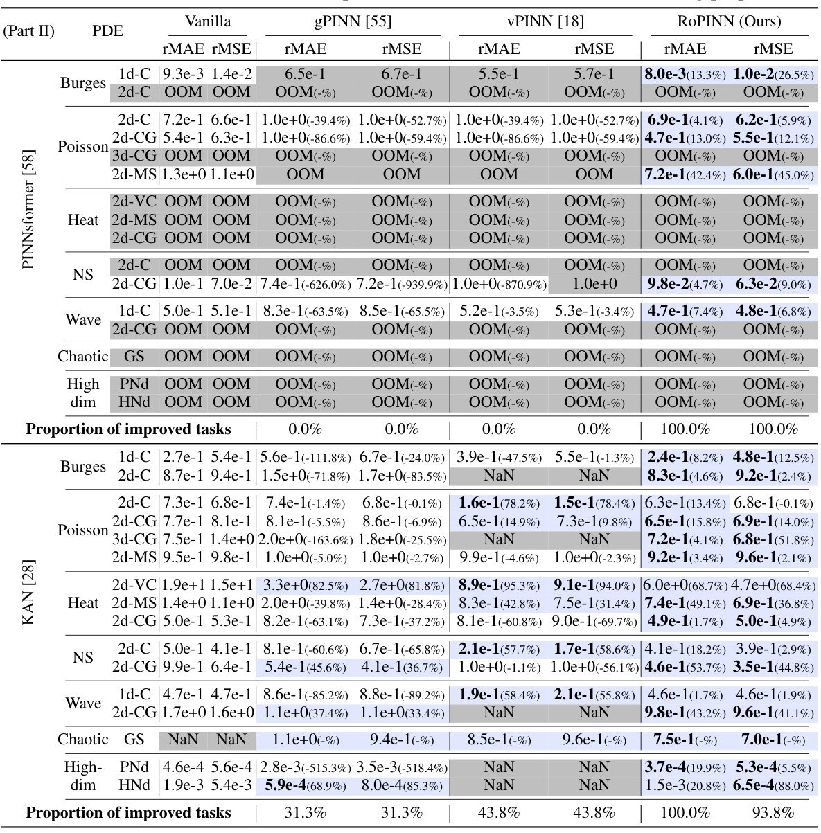
This table compares the performance of RoPINN against gPINN and vPINN across various PINN base models on several benchmark PDEs. It shows the loss (loss function), mean absolute error (MAE), and root mean squared error (RMSE) for each method, highlighting improvements achieved by RoPINN. The results for PINNacle are presented as the percentage of improved tasks out of 16 total tasks.
Full paper#
