↗ OpenReview ↗ NeurIPS Homepage ↗ Chat
TL;DR#
Current selective classification methods suffer from an inherent limitation: they only allow a model to either predict a class or abstain completely, ignoring potentially valuable information when a sample is rejected. This can lead to suboptimal decision-making, particularly in high-stakes scenarios where partial information can still be highly useful. For example, in medical image analysis, rejecting an image that is highly likely to be malignant might result in a delayed diagnosis with potentially dire consequences.
This paper introduces Hierarchical Selective Classification (HSC) as a solution. HSC extends selective classification to handle hierarchical data, allowing models to provide less specific predictions when there’s uncertainty. By using a hierarchical structure of classes, the model can still provide useful information even when it cannot confidently classify to the most specific level. The authors introduce new inference rules for HSC and show that this approach consistently improves both accuracy and confidence calibration. They also demonstrate that specific training regimes significantly improve HSC’s performance.
Key Takeaways#
Why does it matter?#
This paper is crucial because it addresses the limitations of existing selective classification methods by extending them to hierarchical settings. This allows for more nuanced uncertainty handling and improved decision-making in risk-sensitive applications. The proposed approach has significant implications for computer vision and other fields where hierarchical data structures exist, as demonstrated by extensive empirical studies on ImageNet. It also opens up new avenues for research in uncertainty quantification and improved training regimes for hierarchical classification.
Visual Insights#

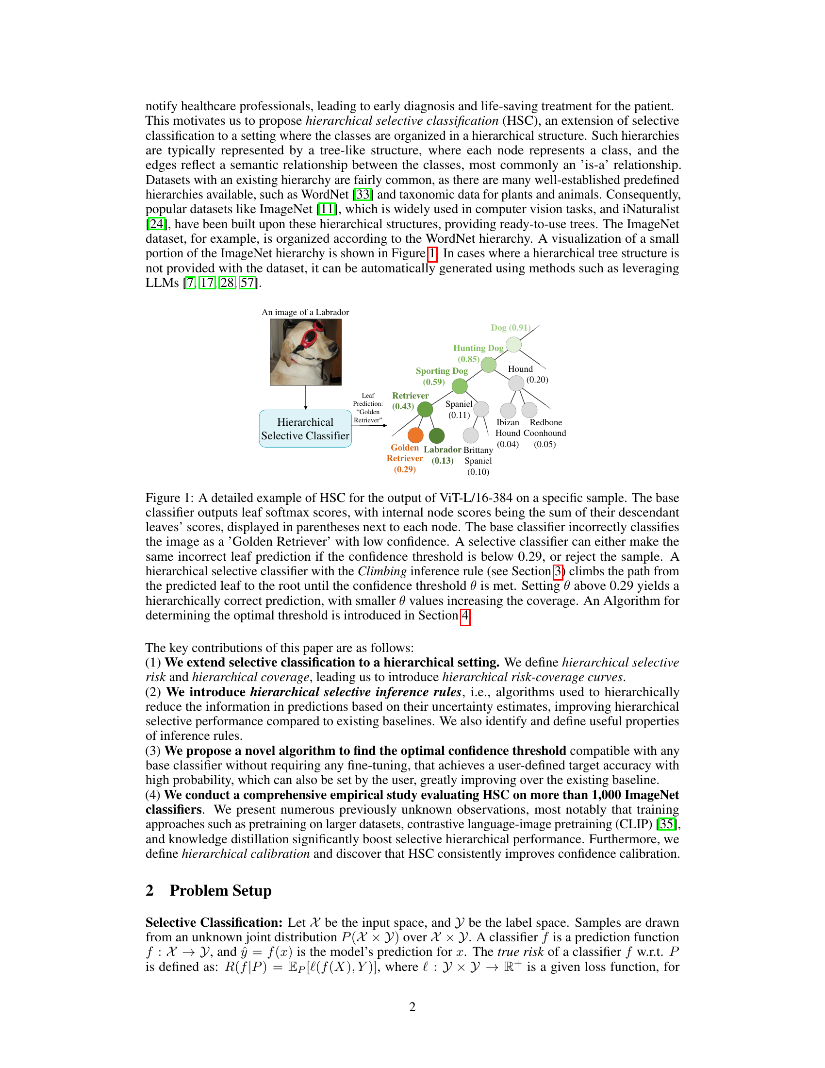
This figure illustrates how Hierarchical Selective Classification (HSC) works using the example of a Labrador Retriever image classified by a ViT-L/16-384 model. The base classifier initially misclassifies the image as a ‘Golden Retriever’ with low confidence. HSC, however, leverages a hierarchical class structure (shown as a tree) to provide a more accurate, higher-level classification (‘Dog’) when uncertainty exists at the leaf node level. The Climbing inference rule is used to ascend the hierarchy until a sufficient confidence threshold is reached, improving both accuracy and coverage.

This table presents a comparison of the performance of three different hierarchical selective inference rules (Selective, Max-Coverage, and Climbing) on two image classification datasets: ImageNet-1k and iNat21. The performance is measured using the hierarchical Area Under the Risk-Coverage curve (hAURC) and the hierarchical gain, representing the improvement in hAURC compared to the standard selective method. The results show that the Climbing inference rule significantly outperforms the other methods on both datasets.
In-depth insights#
Hierarchical Risk#
Hierarchical risk, in the context of a hierarchical classification system, moves beyond the simple binary right/wrong assessment of a single prediction. It introduces a more nuanced evaluation by considering the hierarchical relationship between classes. A misclassification at a higher level of the hierarchy (e.g., mistaking a Labrador for a dog, rather than a specific breed) is generally considered less severe than a misclassification at a lower level (e.g., mistaking a Labrador for a Golden Retriever). This approach acknowledges the inherent uncertainty often present in real-world datasets, where perfect specificity is unlikely. By quantifying the cost of different levels of error, hierarchical risk provides a more realistic evaluation metric for risk-sensitive applications such as medical diagnosis, where some level of uncertainty is acceptable if it leads to the correct higher-level classification. This methodology allows for more fine-grained control and a better understanding of model performance in hierarchical structures. Furthermore, it offers the potential to optimize models for the desired level of specificity versus the tolerance for uncertainty in higher-level classifications.
Inference Rules#
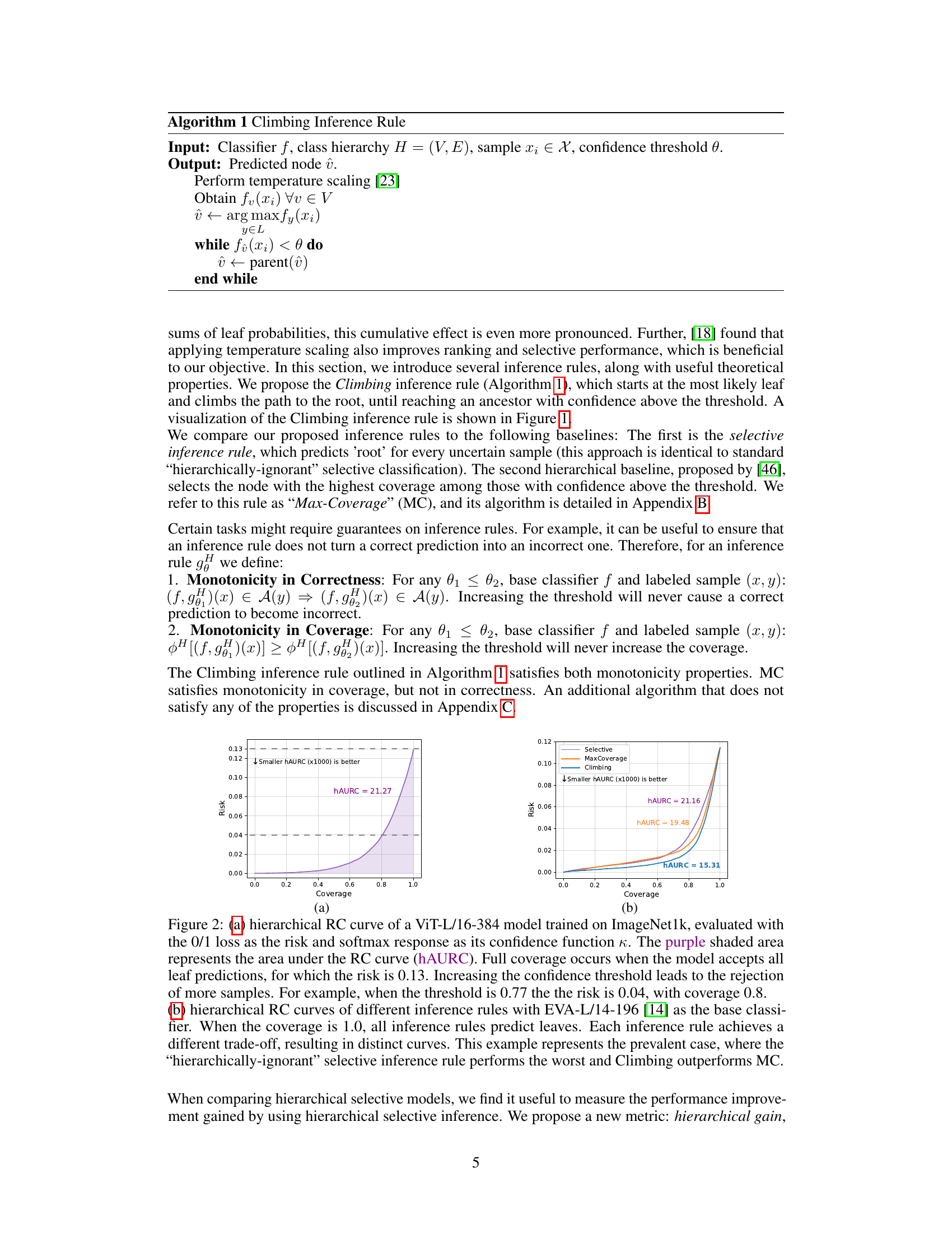
The section on ‘Inference Rules’ is crucial for understanding how the hierarchical selective classification (HSC) model makes predictions. It introduces different algorithms, or rules, governing how the model navigates the class hierarchy when uncertainty is high. The Climbing rule, for instance, starts at the most likely leaf node and ascends the hierarchy until sufficient confidence is reached, offering a balance between accuracy and specificity. Contrastingly, the Max-Coverage rule prioritizes maximizing the coverage of the prediction, potentially sacrificing precision. The choice of inference rule significantly impacts the model’s performance, as demonstrated by the empirical results comparing their respective hierarchical risk-coverage curves (hAURC). The authors also discuss the desirable properties of inference rules, such as monotonicity in correctness and coverage. These properties ensure that increasing the confidence threshold doesn’t transform correct predictions into incorrect ones and never increases coverage. The introduction of these various inference rules is a key contribution, highlighting the flexibility of HSC and its ability to adapt to different task requirements. The optimal rule selection would depend on the trade-off between the risk and coverage desired for a particular task.
Optimal Threshold#
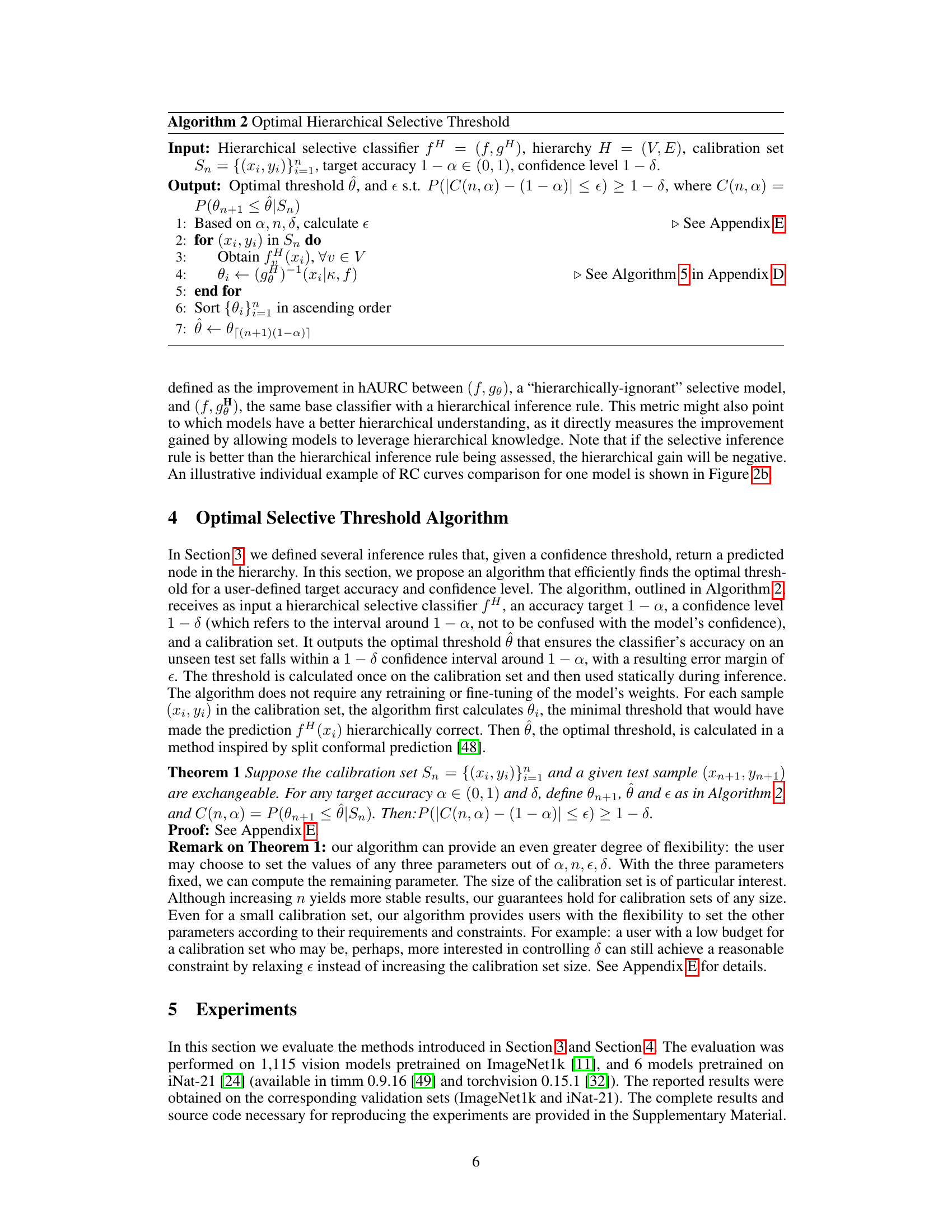
The optimal threshold selection is a crucial aspect of selective classification, aiming to balance model accuracy and coverage. Finding this threshold is computationally challenging, often involving iterative algorithms or complex optimization procedures. The paper explores an algorithm that, given a target accuracy and confidence level, efficiently finds an optimal threshold. This method leverages a calibration set to estimate the threshold’s performance and provides strong theoretical guarantees on achieving the target accuracy with high probability. The algorithm is notable for its efficiency, as it avoids retraining and can adapt to different user-defined parameters. The use of a calibration set separates the training and deployment phases, ensuring that the threshold selection is not overly sensitive to the training data itself. By combining theoretical rigor with practical efficiency, this optimal threshold algorithm makes selective classification more robust and user-friendly.
Training Regimes#
The study’s exploration of training regimes reveals CLIP’s exceptional performance in improving hierarchical selective classification, significantly outperforming other methods like knowledge distillation and pretraining on larger datasets. This suggests that CLIP’s image-text alignment facilitates a deeper semantic understanding, leading to more robust and informative hierarchical predictions. The results also highlight the benefits of pretraining on larger datasets like ImageNet-21k, although the improvement varies across models. Knowledge distillation also shows positive impact, aligning with prior research. Interestingly, using linear probes with CLIP models offers even greater advantages than zero-shot CLIP, emphasizing the importance of careful model fine-tuning for optimal performance in hierarchical selective classification. These findings offer valuable insights for practitioners, guiding choices in training regimes to maximize performance and potentially uncover new training approaches for future research.
Calibration Curve#
Calibration curves are a crucial tool for evaluating the reliability of a classifier’s predicted probabilities. A well-calibrated classifier should produce probabilities that accurately reflect the true frequency of positive outcomes. Deviations from a perfect diagonal line (representing ideal calibration) reveal miscalibration. For instance, an overconfident classifier might yield high probabilities for many negative instances, resulting in a curve above the diagonal. Conversely, an underconfident model might exhibit a curve below the diagonal. Analyzing calibration curves helps identify regions where the model’s probability estimations are particularly unreliable, allowing for targeted improvements through techniques such as temperature scaling or other recalibration methods. Furthermore, the area under the calibration curve (AUC) can be used as a quantitative metric to compare the calibration performance of different models or calibration methods. Different applications may have different tolerance for miscalibration, making this type of analysis vital for risk-sensitive applications like medical diagnosis where confidence estimations are paramount. The shape of the curve provides insights into the nature of miscalibration, which is essential for selecting the appropriate recalibration technique. Ultimately, calibration curves are indispensable for ensuring trustworthy and reliable predictions.
More visual insights#
More on figures

This figure shows two hierarchical risk-coverage (RC) curves. (a) demonstrates a single model’s performance, highlighting the relationship between risk and coverage as the confidence threshold changes. The shaded area represents the hierarchical area under the RC curve (hAURC). (b) compares three different inference rules for hierarchical selective classification using a different base model. It shows how each rule achieves a distinct trade-off between risk and coverage, illustrating the advantages of the ‘Climbing’ rule.

This figure compares the performance of the proposed hierarchical selective threshold algorithm against DARTS for two different models (EVA-Giant/14 and ResNet-152). It visualizes the distribution of accuracy results obtained from 1000 runs of each algorithm for a target accuracy of 95% and a confidence level of 90%. The plots show that the proposed algorithm consistently achieves higher accuracy closer to the target, whereas DARTS either fails to meet the accuracy constraint or leads to zero coverage.
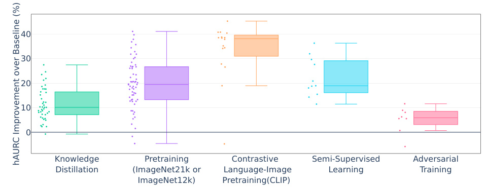
This figure shows a box plot comparing the improvement in hierarchical area under the risk-coverage curve (hAURC) achieved by different training methods (knowledge distillation, pretraining on ImageNet21k or ImageNet12k, contrastive language-image pretraining (CLIP), semi-supervised learning, and adversarial training) relative to a baseline model trained without these methods. The x-axis represents the training method, and the y-axis represents the percentage improvement in hAURC. Each data point represents a single model, and the box plot shows the median, quartiles, and range of improvement for each method.
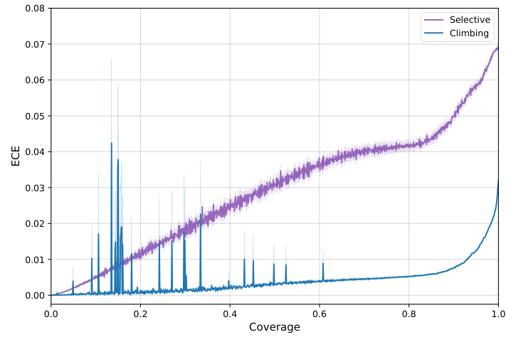
This figure shows the aggregated Calibration-Coverage (CC) curves for 1115 ImageNet models. The CC curves plot the Expected Calibration Error (ECE) against coverage. Two inference rules, Selective and Climbing, are compared; Climbing generally shows better calibration than Selective, indicating that hierarchical selective classification improves calibration.
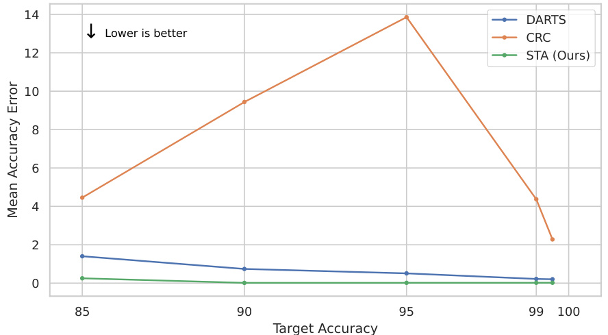
This figure compares the performance of the proposed hierarchical selective threshold algorithm against DARTS using individual model examples. Each algorithm was run 1000 times with a target accuracy of 95% and a confidence level of 90%. The plot shows the mean and median accuracy errors, along with the confidence intervals for each algorithm. The results demonstrate that the proposed algorithm consistently achieves lower accuracy errors and higher coverage compared to DARTS.

This figure compares the hierarchical selective performance of zero-shot CLIP models and their linear-probe counterparts across different backbones. Each point represents a model, with the x-coordinate representing AUROC and the y-coordinate representing -log(hAURC). The round markers show results for zero-shot CLIP models, while the star markers show results for linear-probe CLIP models. The plot shows that linear-probe CLIP models consistently outperform their zero-shot counterparts in terms of both AUROC and hAURC (lower hAURC indicates better performance).
More on tables

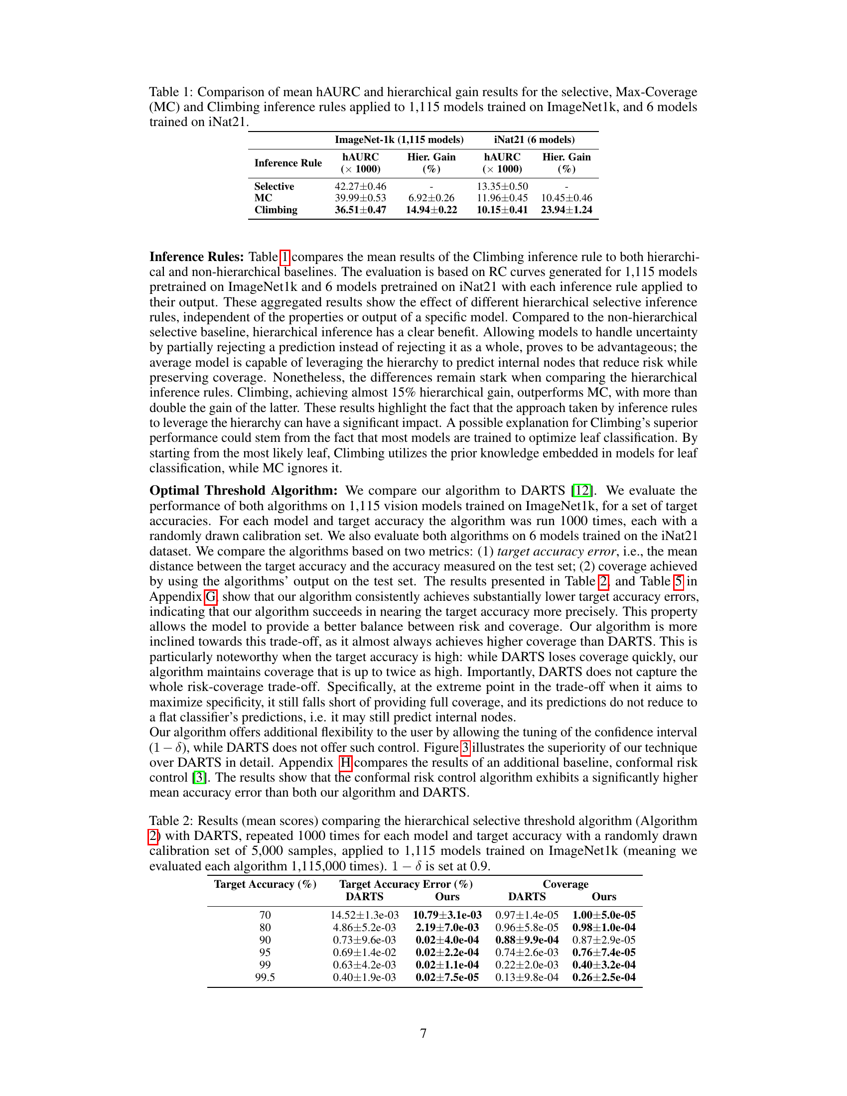
This table presents the results of comparing two algorithms for finding the optimal confidence threshold for hierarchical selective classification. The algorithms are the proposed algorithm (Algorithm 2) and DARTS [12]. The comparison is done across 1,115 ImageNet models, with 1000 runs for each model at various target accuracies. The metrics used for comparison are the target accuracy error and the coverage achieved by each algorithm. Each run uses a randomly selected calibration set of 5000 samples, with a 90% confidence interval (1-δ = 0.9).

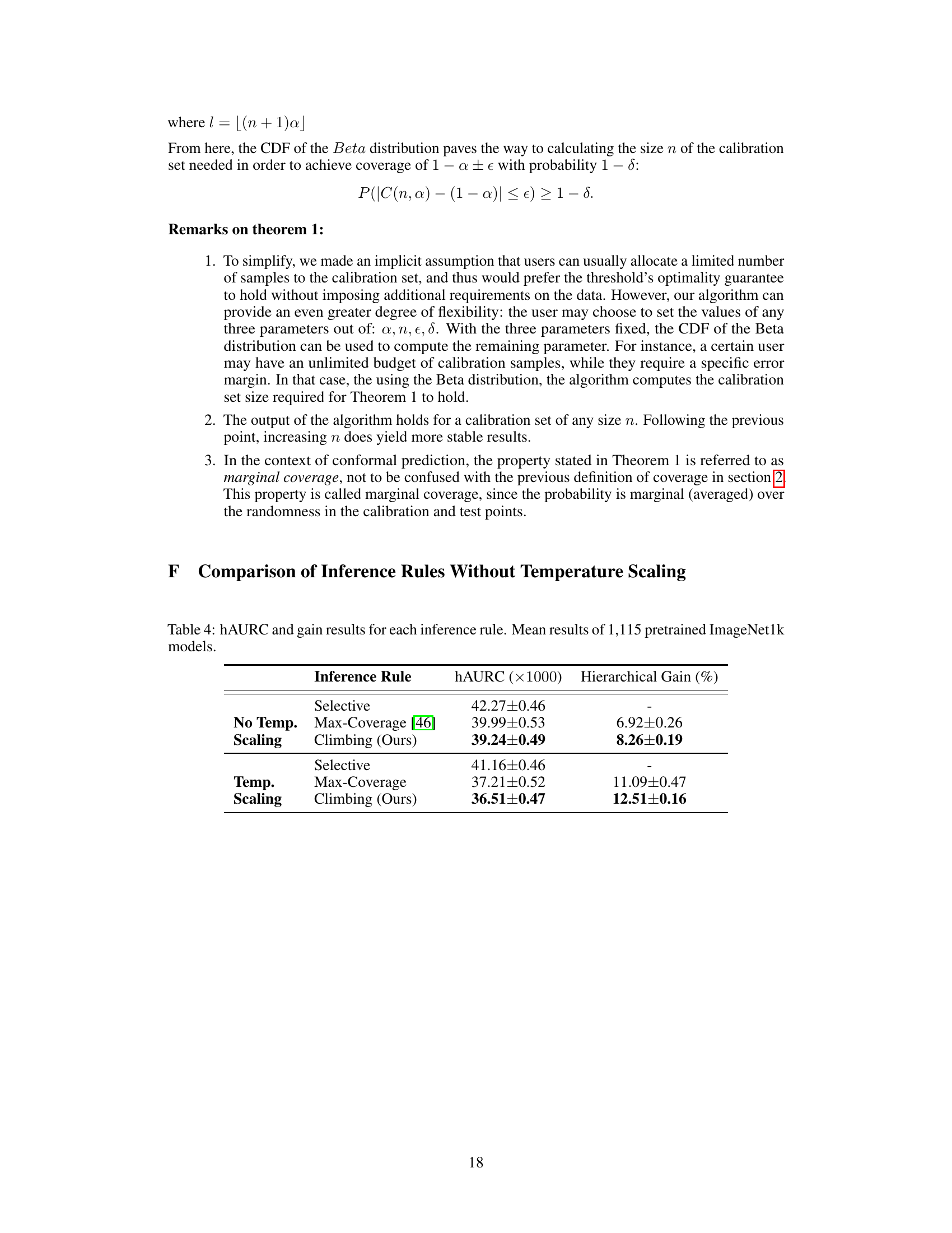
This table presents the results of comparing three different hierarchical selective inference rules (Selective, Max-Coverage, and Climbing) on 1,115 ImageNet1k-trained models. The comparison uses a hierarchical severity risk metric, which takes into account the severity of misclassifications based on their position in the class hierarchy. The table shows the mean hAURC (hierarchical Area Under the Risk-Coverage curve) and the hierarchical gain (the improvement in hAURC compared to the baseline Selective inference rule) for each inference rule.

This table presents a comparison of the hierarchical Area Under the Risk-Coverage curve (hAURC) and hierarchical gain for three different inference rules: Selective, Max-Coverage, and Climbing. The comparison is made across two datasets: ImageNet1k (1115 models) and iNat21 (6 models). The hAURC metric quantifies the performance of hierarchical selective classification, while the hierarchical gain represents the improvement achieved by using hierarchical inference compared to a non-hierarchical approach.

This table presents a comparison of the hierarchical selective classification performance using three different inference rules: Selective, Max-Coverage, and Climbing. The comparison is made across two datasets: ImageNet1k (1115 models) and iNat21 (6 models). For each inference rule, the mean hAURC (hierarchical area under the risk-coverage curve) and the hierarchical gain (percentage improvement compared to the selective baseline) are reported.

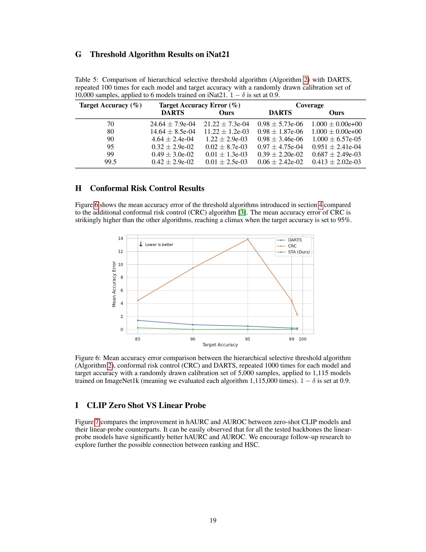
This table compares the performance of the proposed optimal hierarchical selective threshold algorithm (Algorithm 2) against the DARTS algorithm. The comparison is based on two key metrics: target accuracy error and coverage. The results were obtained by running each algorithm 100 times for six models trained on the iNat21 dataset, with each run using a different randomly selected calibration set of 10,000 samples. The confidence level (1-δ) was fixed at 0.9. The table shows the mean and standard deviation for each metric across the 100 runs, for several target accuracies (70%, 80%, 90%, 95%, 99%, and 99.5%).

This table presents the comparison of three different inference rules: Selective, Max-Coverage, and Climbing. The comparison is based on the mean hierarchical Area Under the Risk-Coverage curve (hAURC) and the hierarchical gain (%). The hAURC measures the overall performance of a hierarchical selective classifier, while the hierarchical gain shows the improvement in performance by using a hierarchical approach over a non-hierarchical one. Two datasets are used: ImageNet1k (1,115 models) and iNat21 (6 models), allowing for a broader evaluation of the inference rules’ effectiveness across different models and datasets. The results show Climbing outperforms other inference rules in most cases.
Full paper#

