↗ OpenReview ↗ NeurIPS Homepage ↗ Chat
TL;DR#
Many real-world reinforcement learning (RL) problems involve multiple reward functions, requiring agents to optimize performance across various objectives. Existing RL methods typically focus on a single reward, making them unsuitable for such multi-reward scenarios. Furthermore, designing reward functions can be complex and iterative, highlighting the need for efficient methods to explore policies across different rewards. This necessitates exploring optimal policies for multiple reward functions simultaneously.
This paper addresses this challenge by introducing the Multi-Reward Best Policy Identification (MR-BPI) problem and presenting two novel algorithms: MR-NaS for tabular Markov Decision Processes (MDPs), and DBMR-BPI for deep RL (DRL). MR-NaS leverages a convex approximation of a theoretical lower bound on sample complexity to design an optimal exploration policy. DBMR-BPI extends this approach to model-free exploration in DRL. Extensive experiments demonstrate that these algorithms outperform existing methods in various challenging environments and generalize well to unseen reward functions.
Key Takeaways#
Why does it matter?#
This paper is crucial for researchers in reinforcement learning because it tackles the largely unexplored problem of efficiently identifying optimal policies across multiple reward functions. The proposed algorithms, MR-NaS and DBMR-BPI, offer significant improvements in sample efficiency and generalizability, paving the way for more robust and adaptable AI agents in various real-world applications. Furthermore, the rigorous theoretical analysis provides valuable insights into the fundamental limits of multi-reward exploration, guiding future research in this exciting area.
Visual Insights#

This figure presents the average estimation error of optimal policies across four different environments (Riverswim, Forked Riverswim, DoubleChain, and NArms). The estimation error is calculated as the symmetric difference between the set of optimal policies in the true MDP and the set of optimal policies in the estimated MDP. The figure shows three plots: the first one combines the results for both the canonical basis of rewards and the random rewards, the second one uses only canonical basis rewards, and the third one uses only the random rewards. Shaded areas represent the 95% confidence intervals.

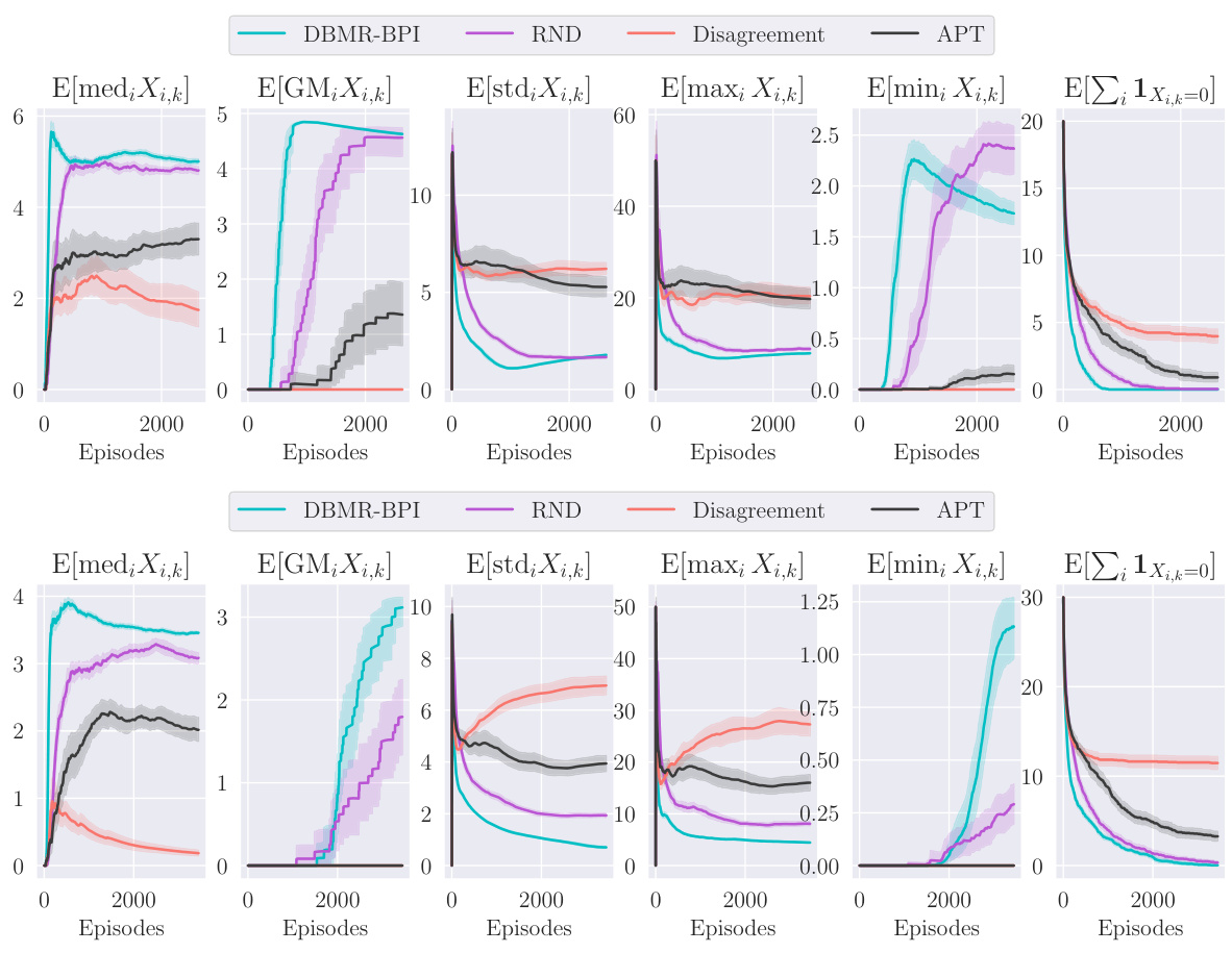
This table presents the results for the Cartpole swing-up experiment. It shows the statistics for the random variable Xᵢ, which is the sum of rewards received when the pole is upright (i.e., satisfying specific conditions). The table compares different algorithms (DBMR-BPI, RND, APT, Disagreement) for different difficulty levels (k = 3, 5) and training steps (T = 150000, 200000). The results are shown as average, standard deviation, minimum, and maximum values of Xᵢ, along with 95% confidence intervals.
In-depth insights#
MR-BPI Lower Bound#
The heading ‘MR-BPI Lower Bound’ suggests a theoretical analysis within a research paper focusing on Multi-Reward Best Policy Identification (MR-BPI). This section likely establishes a fundamental limit on the performance of any algorithm attempting to solve the MR-BPI problem. It probably presents a mathematical theorem proving a lower bound on the number of samples (or interactions with the environment) needed to identify the best policy across multiple reward functions, with a specified confidence level. This lower bound serves as a benchmark; any practical algorithm would require at least this many samples. The derivation likely involves information-theoretic arguments or techniques from optimal decision making, potentially utilizing concepts like change-of-measure arguments. The bound is likely instance-specific, meaning its value depends on the characteristics of the specific Markov Decision Process (MDP) being considered and the set of reward functions. The existence of such a lower bound provides crucial insights into the inherent difficulty of the problem and guides the design of efficient exploration strategies. The lower bound’s tightness (how close to the actual minimum sample complexity it is) is also a significant aspect often explored in such theoretical analyses.
MR-NaS Algorithm#
The heading ‘MR-NaS Algorithm’ suggests a multi-reward best policy identification algorithm. The name implies that this algorithm is probably correct (PC), meaning it provides guarantees on finding the optimal policy within a specified confidence level across multiple rewards. It likely incorporates a navigation and stopping mechanism to efficiently balance exploration and exploitation across the reward space. The ‘NaS’ part likely refers to a similar algorithm like ‘Navigate and Stop’ used in single-reward settings. This implies a structure involving an exploration phase where the algorithm samples to estimate the optimal policy for each reward, followed by a stopping criterion to determine when sufficient evidence has been collected. Convex optimization techniques might be employed to derive an optimal or near-optimal exploration strategy, making it efficient even in complex scenarios with multiple rewards. The algorithm likely handles the exploration-exploitation dilemma efficiently by strategically focusing exploration efforts based on uncertainty estimates regarding the optimal policies for the different rewards.
DBMR-BPI#
The proposed algorithm, DBMR-BPI (Deep Bootstrapped Multi-Reward Best Policy Identification), is designed for efficient exploration in deep reinforcement learning (DRL) environments with multiple reward functions. It addresses the challenge of identifying optimal policies across a set of diverse reward signals, a problem common in practical applications where an agent’s objective is multifaceted. DBMR-BPI builds on the foundation of model-based methods by adapting the generative solution of a convex upper bound to the sample complexity lower bound, making it suitable for model-free exploration. The key innovation lies in its capability to handle parametric uncertainty in the estimation of model-specific quantities (such as sub-optimality gaps) inherent in DRL, enhancing the robustness and sample efficiency. Moreover, DBMR-BPI strategically balances exploration across different rewards, dynamically prioritizing those rewards where uncertainty is higher to ensure fast convergence. Its effectiveness is demonstrated through empirical results on challenging benchmarks, showing competitive performance against established unsupervised RL algorithms.
Tabular MDP Results#
In a research paper focusing on multi-reward best policy identification (MR-BPI), a section dedicated to ‘Tabular MDP Results’ would present empirical findings from experiments conducted on tabular Markov Decision Processes (MDPs). This section would likely showcase the performance of the proposed MR-BPI algorithm compared to existing baselines in various tabular MDP environments. Key aspects to look for would include sample efficiency, demonstrated by the number of steps needed to identify optimal policies, generalization capabilities, showing the algorithm’s ability to perform well on unseen reward functions, and robustness, evaluating the performance under different experimental settings and various levels of difficulty. The results would be presented in a clear and organized manner using tables and figures to highlight key comparisons and trends. A detailed analysis of the results would help to draw conclusions about the strengths and weaknesses of the proposed approach in simpler, tabular MDP settings, and inform its potential scalability to more complex, deep reinforcement learning scenarios.
Deep RL Results#
A hypothetical ‘Deep RL Results’ section would likely present empirical findings from applying deep reinforcement learning (DRL) algorithms to complex control tasks. The results would ideally show how the DRL agent learns and performs compared to baselines (e.g., existing methods). Key metrics might include the cumulative reward accumulated over time, the learning curve (reward vs. timesteps), and a comparison of success rates or completion times across different tasks or environments. The section would benefit from an analysis of the agent’s learning process, including exploration strategies employed and the representation learned by the model. Visualizations, such as graphs and plots, would be crucial to illustrate the findings effectively and provide insightful comparisons between different methods. Furthermore, the discussion should explain potential limitations of the DRL approach. A critical assessment should include factors like sample efficiency, sensitivity to hyperparameters, computational cost, and the generalizability of results to unseen scenarios. Finally, a broader discussion connecting the empirical results to relevant theoretical work, highlighting the algorithm’s strengths and weaknesses in light of existing DRL theory, would provide significant value.
More visual insights#
More on figures

This figure shows a simple Markov Decision Process (MDP) with two states and two actions, along with a plot illustrating the minimum sub-optimality gap. The MDP is represented as a graph, where each edge shows an action, its transition probability, and the reward received. The reward function depends on a parameter θ (theta), and its minimum sub-optimality gap demonstrates the non-convexity and discontinuity issues in the multi-reward best policy identification problem.

This figure shows a diagram of the Forked Riverswim environment. It’s a variation of the standard Riverswim environment, designed to be more challenging for exploration algorithms. Unlike the linear chain of states in the standard Riverswim, the Forked Riverswim has branching paths. The agent starts in state s0 and can move left (upstream), or right (downstream) in the main chain or choose to move to a different path at intermediate stages. The tuple (a,p) associated with each transition indicates that action a is taken with probability p. This environment increases the sample complexity and tests an agent’s ability to generalize across different paths within the environment.

The Forked Riverswim environment is a variation of the traditional Riverswim environment, designed to test more complex exploration strategies. In this variant, the state space branches into multiple paths, resembling a river that forks. At intermediate states the agent can switch between the forks, while the end states are not connected. This variant requires the agent to make more sophisticated decisions to explore the environment. This setup increases the sample complexity and challenges the agent’s ability to generalize across different paths within the environment.
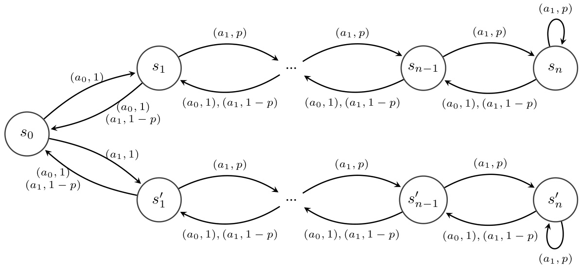
The figure shows a diagram of the Double Chain environment, a reinforcement learning benchmark. It consists of two separate chains of states, unlike the Forked Riverswim environment. The agent cannot transition between the chains, and intermediate states are transient. Each state has two actions: one moving towards the end of the chain (probability p) and one moving towards the start of the chain (probability 1-p). The figure visually represents the states as nodes and the actions and transition probabilities as labeled edges.
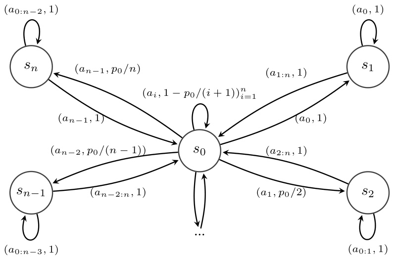
This figure depicts the NArms environment, a simplified version of the 6Arms environment. The environment is a Markov Decision Process (MDP) with n+1 states. The agent starts in state s0 and chooses one of n actions (arms) a0,…,an-1. Each action transitions the agent to state si with probability pi, where pi is defined by a parameter p0. The figure shows the state transition probabilities, indicating the action and its corresponding transition probability. The probability of remaining in state s0 is 1 - p0/(i+1) except for action a0, where it’s 0. This environment challenges the agent’s exploration capabilities due to unequal transition probabilities for each action.

This figure shows the policy estimation error for four different environments (Riverswim, Forked Riverswim, DoubleChain, NArms) using four different algorithms (MR-NaS, RF-UCRL, ID3AL, MR-PSRL). The error is calculated as the symmetric difference between the set of optimal policies in the true MDP and the set of optimal policies in the estimated MDP. Three plots are provided, each showing the error over different reward sets. The first combines the canonical basis rewards and random rewards, while the second and third show results for the canonical and random rewards alone, respectively.
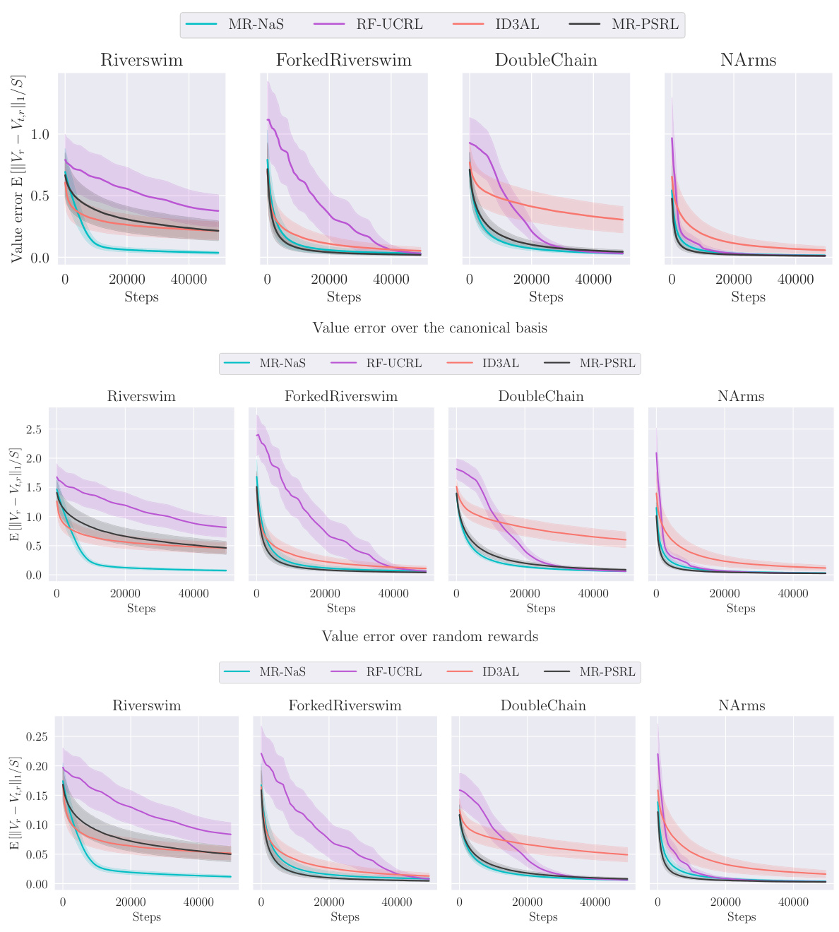
The figure displays the average estimation error of optimal policies for three different reward settings. The error is calculated as the symmetric difference between the sets of optimal policies in the true MDP and the estimated MDP. The three plots show the error for: (1) both the canonical basis of rewards and randomly generated rewards, (2) only the canonical basis, and (3) only the randomly generated rewards. Each plot shows results for four environments: Riverswim, Forked Riverswim, DoubleChain, and NArms. The shaded areas represent the 95% confidence intervals, indicating uncertainty in the average error.

This figure displays the average deviation in visitation time across different states for four different environments (Riverswim, Forked Riverswim, DoubleChain, and NArms). The deviation, Avisit,t, is calculated as the difference between the maximum and minimum times that the algorithm has visited any state up to time t. It measures how much the algorithm favors some states over others during exploration. Smaller values indicate more uniform exploration across the state space.
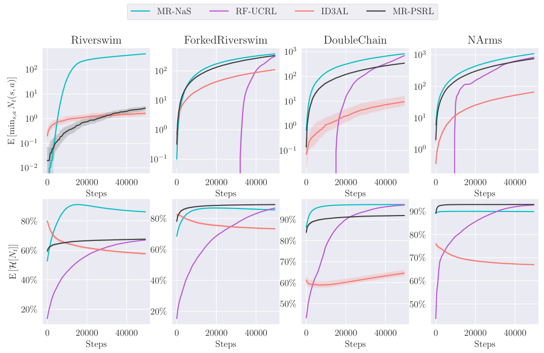
This figure compares four different reinforcement learning algorithms (MR-NaS, RF-UCRL, ID3AL, and MR-PSRL) across four different environments (Riverswim, Forked Riverswim, DoubleChain, and NArms). The top row shows the average number of times the least visited state-action pair was visited over time, illustrating the exploration behavior of each algorithm. The bottom row displays the normalized entropy of the number of state-action visits over time, providing a measure of how evenly each algorithm explores the state-action space. The plots show how the different algorithms explore different aspects of the environments and the trade-off between exploration and exploitation.

The Cartpole swing-up problem involves balancing a pole attached to a cart on a frictionless track. The cart’s position is controlled by applying force, and the goal is to swing the pole up from a hanging position and maintain its balance. This is a challenging reinforcement learning problem due to the sparsity of the reward signal (reward is only obtained when the pole is balanced), and the penalty for movement. The figure illustrates the setup, showing the cart, pole, angle (θ), angular velocity (θ̇), and the goal position of the upright pole.

This figure presents the results of policy estimation error for four different environments: Riverswim, Forked Riverswim, DoubleChain, and NArms. Three plots are shown, each comparing the performance of four different algorithms (MR-NAS, RF-UCRL, ID3AL, and MR-PSRL) in estimating optimal policies. The first plot combines results using both the canonical basis rewards and random rewards, while the second and third plots show results using only canonical basis rewards and random rewards, respectively.

The figure presents the policy estimation error over different sets of rewards and environments. It shows the average value of et,r (the symmetric difference between the set of optimal policies in the true MDP and the estimated MDP) and its 95% confidence interval. The first plot combines the results for the canonical basis of rewards and random rewards, while the other two plots consider each set separately. The results demonstrate that MR-NaS outperforms the baselines in estimating optimal policies, particularly when focusing on the canonical basis of rewards.
This figure shows the policy estimation error of the Multi-Reward Navigate and Stop (MR-NaS) algorithm and three baselines (RF-UCRL, ID3AL, and MR-PSRL) across four different environments (Riverswim, Forked Riverswim, DoubleChain, and NArms). The error is calculated as the symmetric difference between the set of optimal policies in the true MDP and the estimated MDP. Three plots are shown, corresponding to (1) combining the results for canonical and random rewards, (2) using only canonical rewards, and (3) only using random rewards. The figure displays the mean and 95% confidence intervals for each algorithm across 100 seeds.

This figure shows the average estimation error for four different environments (Riverswim, Forked Riverswim, DoubleChain, and NArms) across four different algorithms (MR-NAS, RF-UCRL, ID3AL, and MR-PSRL). The x-axis represents the number of steps taken. The y-axis represents the average estimation error, showing how frequently the algorithms incorrectly identified the optimal policy. Shaded regions denote 95% confidence intervals based on 100 independent simulation runs. This illustrates the relative performance of the algorithms in terms of accurately identifying the best policy for a given reward function, with MR-NaS generally showing superior performance.

This figure displays the average estimation error of the optimal policies over time steps for four different environments (Riverswim, Forked Riverswim, DoubleChain, and NArms) and four different algorithms (MR-NaS, RF-UCRL, ID3AL, and MR-PSRL). The shaded region represents the 95% confidence interval calculated from 100 independent runs. Each plot shows the average estimation error for each algorithm across the various time steps in the corresponding environment. The x-axis denotes the number of steps performed by the algorithms, and the y-axis shows the average estimation error. The different colours and lines denote different algorithms.
This figure shows the estimation error of optimal policies for different reward sets and algorithms. The plots show the average value of et,r, which represents the symmetric difference between the optimal policy sets of the true MDP and the estimated MDP at time t, for a given reward r, along with 95% confidence intervals. The figure includes three subplots showing results for the canonical basis, the random rewards and a combination of both. This helps evaluate the algorithms’ performance in various scenarios.
The figure displays the average estimation error for the optimal policies across various hard exploration tabular environments. The error is calculated as the symmetric difference between the set of optimal policies in the true MDP and the set of optimal policies in the estimated MDP. The figure compares the performance of MR-NAS against three baselines (RF-UCRL, ID3AL, and MR-PSRL) across three different reward allocation scenarios: 1) Canonical basis rewards combined with random rewards; 2) canonical basis rewards only; and 3) random rewards only. The results show the average estimation error, as well as 95% confidence intervals, over 100 seeds, for a specified number of steps.
This figure displays the average estimation error of optimal policies across four different environments (Riverswim, Forked Riverswim, DoubleChain, and NArms) and four different algorithms (MR-NaS, RF-UCRL, ID3AL, and MR-PSRL). The error is calculated as the symmetric difference between the set of optimal policies in the true MDP and the estimated MDP. The shaded areas represent 95% confidence intervals, based on 100 independent runs. The figure shows the error over time (number of steps).

This figure displays the average estimation error of the optimal policies over time steps for four different environments: Riverswim, Forked Riverswim, DoubleChain, and NArms. The error is calculated as the symmetric difference between the set of optimal policies in the true MDP and the set of optimal policies in the estimated MDP. The shaded area shows the 95% confidence intervals based on 100 independent runs of each algorithm for each environment. The plot shows the algorithms’ progress in accurately identifying the optimal policies. Note that the reward r is a random variable.
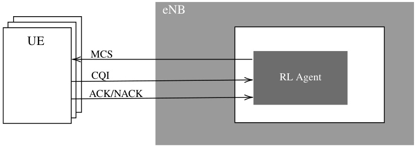
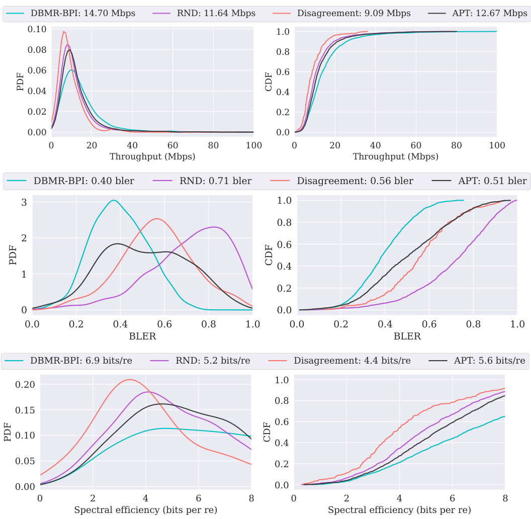
The figure shows a diagram of a downlink link adaptation system. It shows multiple UEs transmitting data to an eNB (evolved NodeB) via a wireless link. The RL agent at the eNB receives CQI (Channel Quality Indicator) feedback and ACK/NACK (Acknowledgement/Negative Acknowledgement) indicating successful/failed data transmissions from the UEs. Based on the received feedback, the RL agent dynamically adjusts the MCS (Modulation and Coding Scheme) for transmission. The MCS determines the transmission rate and reliability, thus balancing throughput, spectral efficiency, and reliability.
This figure presents the average estimation error for four different environments (Riverswim, Forked Riverswim, DoubleChain, and NArms) across four different algorithms (MR-NaS, RF-UCRL, ID3AL, and MR-PSRL). The estimation error is calculated over T time steps and considers a random reward r. Shaded regions represent 95% confidence intervals across 100 independent experimental runs. The figure shows the performance of MR-NaS compared to other baseline methods across various environments.

This figure shows the estimation error of the optimal policies for four different environments: Riverswim, Forked Riverswim, DoubleChain, and NArms. The estimation error is calculated as the symmetric difference between the set of optimal policies in the true MDP and the set of optimal policies in the estimated MDP. The figure shows three different plots, one for each of the three sets of rewards used in the experiments: canonical rewards, random rewards, and a combination of both.

This figure displays the average estimation error over a series of time steps (t) for four different hard-exploration tabular environments: Riverswim, Forked Riverswim, DoubleChain, and NArms. The error is calculated for each environment using four different algorithms: MR-NaS, RF-UCRL, ID3AL, and MR-PSRL. The shaded area represents the 95% confidence interval, calculated from 100 independent runs, making the results statistically robust. Each plot shows how the estimation error decreases as the number of steps increases, indicating the convergence of the algorithms. The comparison allows for evaluation of the relative efficiency of each algorithm in identifying optimal policies across the different environments.

This figure shows the average estimation error of optimal policies over time steps for four different environments: Riverswim, Forked Riverswim, DoubleChain, and NArms. The error is calculated as the symmetric difference between the set of optimal policies in the true MDP and the estimated MDP. The shaded area represents the 95% confidence interval based on 100 independent simulation runs. The figure helps illustrate how the different algorithms perform in identifying optimal policies across different environments, highlighting the speed and accuracy of convergence.
More on tables

The table presents the results for two difficulty levels (k=3,5) and various training steps (T=150000, 200000). The random variable Xᵢ represents the sum of positive rewards accumulated by the agent up to time T. For each reward in the set Rbase (base rewards), the table shows the mean, standard deviation, median, maximum, and minimum values of Xᵢ, averaged across 30 independent seeds. Statistically significant results are highlighted in bold.

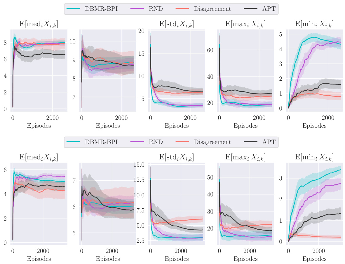
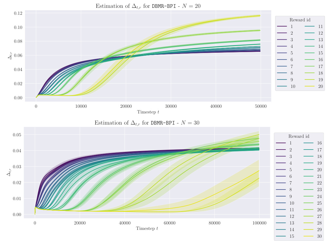
This table presents the performance of different algorithms (DBMR-BPI, RND, APT, Disagreement) on the DeepSea environment for different sizes of the grid (N=20 and N=30). For each algorithm, the table shows the average reward collected (E[AvgR({Xi})], E[AvgRnd({Xi})]), standard deviation (E[stdr({Xi})], E[stdRnd({Xi})]), median (E[medR({Xi})], E[medRnd({Xi})]), maximum (E[maxR({Xi})], E[maxRnd({Xi})]), minimum (E[minR({Xi})], E[minRnd({Xi})]) and number of cells in the last row of the grid that have not been visited by the algorithm at the end of the experiment (E[∑₁₁ xᵢ=0]). The results are for both the base rewards (R) and random unseen rewards (Rrnd) and are averaged over 30 seeds. Statistically significant results are bolded and the 95% confidence interval is reported in parentheses.
This table presents the numerical results for the Cartpole swing-up problem. The results are averaged over 30 seeds, and the 95% confidence intervals are shown in parentheses. The table shows the average (E[Avg]), standard deviation (E[std]), median (E[med]), minimum (E[min]), and maximum (E[max]) values for the random variable Xᵢ, which represents the sum of rewards received when the pole is upright, across multiple rewards. The results are shown for both the base rewards (R) and randomly generated rewards (Rrnd). Statistically significant results are highlighted in bold.

This table presents the results for the Cartpole swing-up task, comparing the performance of different algorithms (DBMR-BPI, RND, APT, and Disagreement) across two difficulty levels (k=3 and k=5). The values represent statistics for the random variable Xi, which is the sum of rewards received when the pole is upright (or above a certain threshold). The table shows the average (AvgR), median (medR), standard deviation (stdR), maximum (maxR), and minimum (minR) values of Xi, along with 95% confidence intervals. The results highlight the relative performance of DBMR-BPI in accumulating positive rewards compared to the other methods.

This table presents the results of the Cartpole swing-up experiment for different difficulty levels (k=3 and k=5) and training steps (T=150000 and T=200000). The results are averaged over 30 seeds. The key metric is Xᵢ, representing the sum of positive rewards (rᵢ(sₜ, aₜ)) received up to time T, where rᵢ is drawn from the set of random rewards Rrnd (not used during training). The table shows statistical measures (mean, median, standard deviation, maximum, and minimum) for Xᵢ, highlighting statistically significant differences using bold font and confidence intervals in parentheses.

This table lists the hyperparameters used for each of the algorithms evaluated in the paper. The hyperparameters are divided into categories by algorithm (DBMR-BPI, APT, Disagreement, RND) and then lists the specific value assigned to each parameter within each algorithm. Note that all algorithms used a batch size of 128.

This table presents the statistical results for the DeepSea environment, focusing on the random variable Xᵢ, which represents the sum of rewards obtained for the i-th reward in a specific instance. The results are averaged across 30 seeds, with values multiplied by 100 and rounded to the first digit. 95% confidence intervals are included in parentheses. The table includes statistics such as the median, geometric mean, standard deviation, maximum, minimum, and the sum of instances where Xᵢ equals zero. These metrics provide insights into the performance of various algorithms across different rewards in the DeepSea environment.

This table presents the results for the Cartpole swing-up problem, focusing on the random rewards. The random variable Xᵢ represents the sum of positive rewards collected by the agent during each episode. The table shows the average, standard deviation, median, maximum, and minimum values of Xᵢ for different algorithms (DBMR-BPI, RND, APT, Disagreement) and difficulty levels (k=3 and k=5). Statistically significant results are highlighted.

This table lists the hyperparameters used for each algorithm in the Deep Reinforcement Learning experiments. It shows the values used for DBMR-BPI, APT, Disagreement, and RND, including parameters such as ensemble size, network architecture, learning rates, exploration parameters, and buffer size. The consistent batch size of 128 is also noted.

This table lists the hyperparameters used for each of the algorithms in the experiments: DBMR-BPI, APT, Disagreement, and RND. It shows the values used for parameters such as ensemble size, network architecture, learning rates, and other algorithm-specific settings. The batch size was consistently set to 128 across all algorithms.

This table presents the numerical results for the Cartpole swing-up problem, comparing the performance of DBMR-BPI against several baselines. The results show the average, standard deviation, minimum, and maximum of the random variable X₁, which is the sum of rewards received when the pole is upright from time step 1 to T. The table is divided into sections for different difficulty levels (k) and training steps (T), with both base and randomly generated rewards.
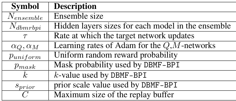
This table lists the hyperparameters used for each of the algorithms evaluated in the paper. It includes the values for DBMR-BPI (Deep Bootstrapped Multi-Reward BPI), RND (Random Network Distillation), APT (Auxiliary Prediction Target), and Disagreement. The hyperparameters control various aspects of each algorithm’s learning process, such as network architecture, learning rates, and exploration strategies. The consistent batch size of 128 is also noted.

This table lists the hyperparameters used for the different algorithms in the Deep Reinforcement Learning experiments. It includes details for DBMR-BPI, RND, APT, and Disagreement algorithms. The table shows the values for parameters such as network architecture (Nensemble, Ndbmrbpi, Ndqn, Ntrunk, Ndisag, Nrnd, NF, NB), learning rates (α, αr, αμ, lapt, Arnd), exploration parameters (Puniform, Pmask), and the size of the replay buffer (C). A batch size of 128 was used consistently across all algorithms.

This table presents the hyperparameters used for all the algorithms in the experiments. It shows the values used for DBMR-BPI, RND, APT, and Disagreement, including specifics like ensemble size, network layer sizes, learning rates, and other algorithm-specific parameters. A batch size of 128 was consistently used across all algorithms.

This table lists the hyperparameters used for all algorithms in the experiments. The table includes values for DBMR-BPI, RND, APT, and Disagreement, showing the specific values set for various parameters such as ensemble size, network architecture, learning rates, exploration parameters, and more.

This table lists the hyperparameters and their values used for the different algorithms evaluated in the paper. It includes details for DBMR-BPI, RND, APT, and Disagreement, specifying values for parameters such as network architecture, learning rates, exploration factors, and other algorithm-specific settings. The consistent batch size of 128 is also noted.
Full paper#

