↗ OpenReview ↗ NeurIPS Homepage ↗ Chat
TL;DR#
Current neural network models often lack robustness when dealing with out-of-distribution (OOD) data—data that differ significantly from the training data. This paper tackles this critical issue by focusing on improving uncertainty quantification. Existing methods rely on strong assumptions about the data distribution, limiting their applicability and accuracy.
This work introduces a novel, non-parametric method that addresses the limitations of current approaches. By combining Lens Depth and Fermat distance, it provides a more accurate uncertainty score directly in the feature space without requiring distributional assumptions or model retraining. The method demonstrates superior performance on multiple datasets, offering a significant advancement in OOD detection and reliable prediction for safety-critical systems.
Key Takeaways#
Why does it matter?#
This paper is crucial for researchers working on uncertainty quantification in machine learning, especially in areas like out-of-distribution (OOD) detection. Its non-parametric, non-intrusive approach and improved accuracy on benchmark datasets offer a valuable solution to existing challenges, offering potential improvements to safety-critical applications and opening new avenues for research in uncertainty estimation and OOD detection.
Visual Insights#

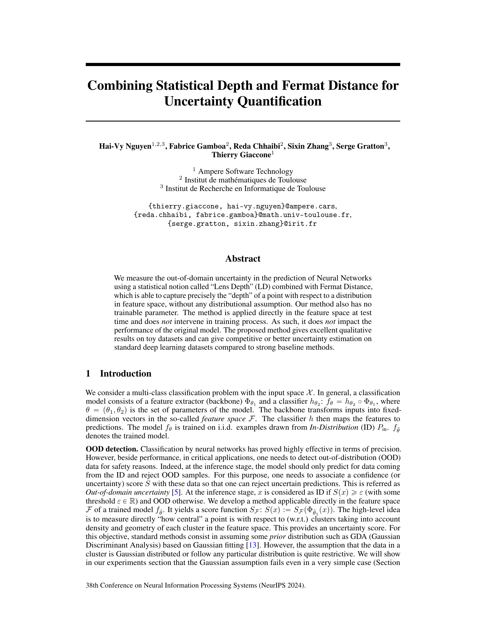
The figure demonstrates the proposed method’s workflow. (a) shows the two-moons dataset where GDA fails to capture the distribution, highlighting the need for a non-parametric approach. (b) illustrates the general scheme. A feature extractor processes inputs (X), creating features (Φθ₁(X) ∈ F). These features are used to compute the Fermat distance and then the Lens Depth, resulting in an uncertainty score S that determines whether a prediction is in-distribution (ID) or out-of-distribution (OOD).

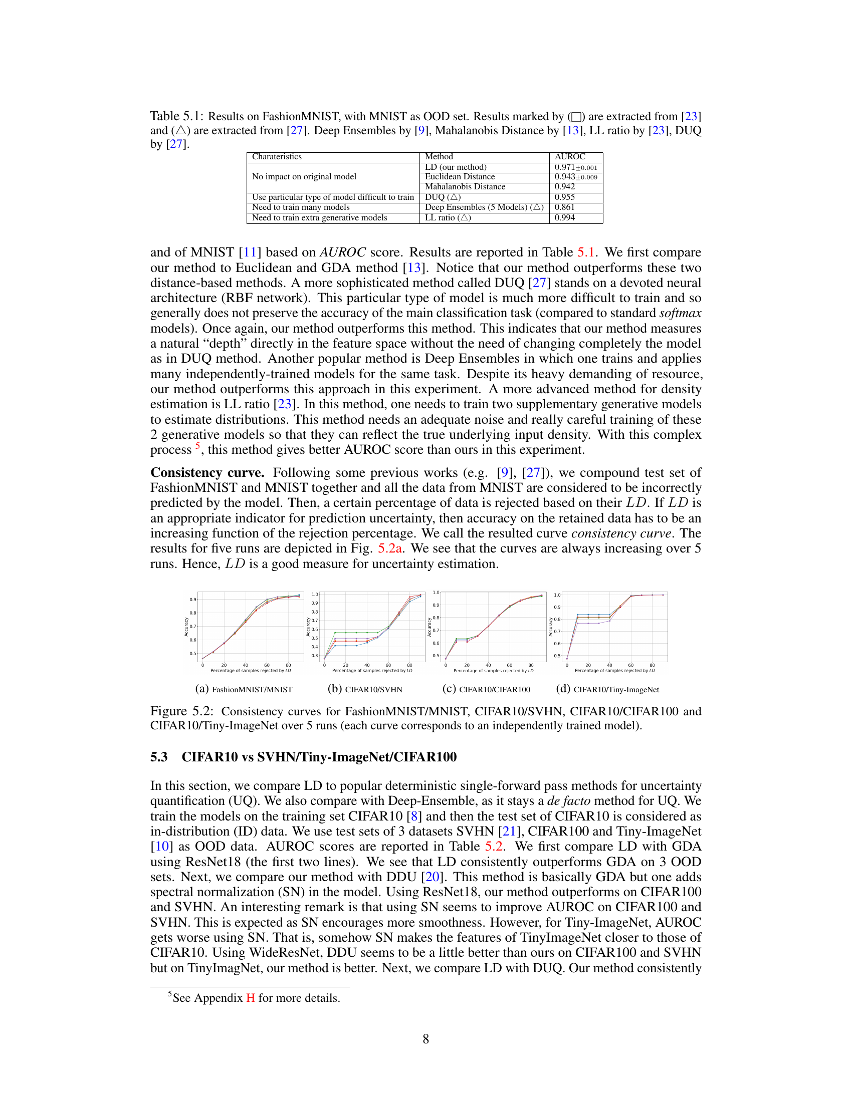
This table compares the performance of different methods for out-of-distribution (OOD) detection on the FashionMNIST dataset using MNIST as the OOD dataset. The table shows the AUROC (Area Under the Receiver Operating Characteristic curve) score for each method. The characteristics of each method are also listed, including whether it impacts the original model, requires specific model types that are difficult to train, needs to train multiple models or extra generative models. The LD (Lens Depth) method proposed in the paper is compared to baseline methods, highlighting its non-intrusive nature and superior performance.
In-depth insights#
Fermat Dist. Depth#
The concept of “Fermat Dist. Depth” merges two powerful ideas: Fermat distance and statistical depth. Fermat distance, unlike Euclidean distance, intelligently adapts to the underlying data distribution’s geometry and density, finding shortest paths that prioritize high-density regions. This is crucial for accurately capturing the shape of complex clusters, overcoming limitations of traditional methods that assume simple, often Gaussian, distributions. Statistical depth functions, in this case, likely lens depth, quantify how ‘central’ a data point is within the distribution. The combination produces a powerful uncertainty quantification metric. Fermat Dist. Depth is non-parametric, meaning it doesn’t rely on strong distributional assumptions. This makes it robust and applicable to a wider range of datasets. The method’s effectiveness relies on choosing an appropriate parameter (alpha) which controls the Fermat distance’s sensitivity to density. A higher alpha value emphasizes density more. However, high alpha values can introduce computational costs that need careful management. In essence, Fermat Dist. Depth offers a novel, flexible, and robust approach to uncertainty quantification in complex data settings by skillfully combining geometric insights from Fermat distance with the probabilistic intuition of statistical depth.
OOD Uncertainty#
The concept of ‘OOD Uncertainty’ in the context of a research paper likely revolves around quantifying the uncertainty associated with predictions made by a model on Out-of-Distribution (OOD) data. The core challenge lies in reliably distinguishing between genuine uncertainty (due to inherent noise or complexity in the data) and uncertainty stemming from the model’s inability to generalize to unseen data points. This is crucial for building robust and safe AI systems, particularly in high-stakes domains. The paper likely explores techniques to estimate this OOD uncertainty, possibly using non-parametric approaches to avoid assumptions about the data distribution. A key focus might be on evaluating the performance of these uncertainty estimation methods, using metrics such as AUROC. The evaluation likely assesses how well these methods discriminate between in-distribution (ID) and OOD data. The research may also investigate the effect of architectural choices or training procedures on OOD uncertainty estimation, aiming to demonstrate a method’s effectiveness on various datasets. Finally, limitations and potential artifacts of the methods are likely discussed, providing a comprehensive understanding of both the strengths and weaknesses of the approaches presented for quantifying OOD uncertainty.
Non-parametric UQ#
Non-parametric uncertainty quantification (UQ) methods are crucial for reliable machine learning, especially when dealing with complex, real-world data where distributional assumptions often fail. Unlike parametric UQ approaches that assume specific probability distributions (e.g., Gaussian), non-parametric methods are more flexible and data-driven. They directly estimate uncertainty from the data without making restrictive assumptions about its underlying structure. This makes them robust to outliers and various data patterns that violate the assumptions of parametric models. Key strengths include their adaptability to diverse datasets and their resistance to model misspecification bias. However, non-parametric UQ often comes with increased computational complexity and challenges in interpretation, potentially requiring sophisticated algorithms and careful consideration of model selection. The effectiveness of non-parametric UQ hinges on the quality of the chosen methods and the data’s inherent characteristics. Therefore, careful selection and validation are vital for obtaining reliable and meaningful uncertainty estimations.
Model-agnostic Score#
A model-agnostic score, in the context of out-of-distribution (OOD) detection, is a crucial component for evaluating the uncertainty of a model’s predictions. Its strength lies in its independence from the specific model architecture; it can be applied to various models (e.g., neural networks, SVMs) without requiring retraining or modification. This feature makes it versatile and widely applicable. The score should ideally reflect the model’s confidence or uncertainty, enabling the identification of data points that fall outside the model’s training distribution. A good model-agnostic score should be highly reliable and robust providing consistent results across different models and datasets. It should effectively capture the uncertainty inherent in model predictions, distinguishing between confident and uncertain predictions. Moreover, a successful model-agnostic score should be computationally efficient to avoid long processing times, and easily interpretable, providing valuable insights into the reasons for uncertainty. Ideally, the score should facilitate effective OOD detection, leading to better safety and reliability in applications where trust in model predictions is paramount.
Small-data Regime#
The concept of a ‘small-data regime’ in machine learning signifies scenarios where the available data for training a model is limited. This poses several challenges. Generalization ability suffers as models trained on small datasets may overfit, performing exceptionally well on the training data but poorly on unseen data. Robustness becomes an issue as the model may not have encountered sufficient variability in the data to handle unexpected inputs effectively. Uncertainty quantification is crucial but can be harder to estimate accurately with limited data. Model selection becomes more difficult, as the limited data may not reveal the optimal model architecture or hyperparameters. Therefore, methods designed for small-data regimes often prioritize regularization techniques to prevent overfitting, and focus on techniques that maximize information extraction from the limited dataset. These techniques may include data augmentation, transfer learning from larger datasets, careful feature engineering, and Bayesian approaches that explicitly model uncertainty. The development of new algorithms optimized for limited data, as well as principled methods to effectively quantify uncertainty, remain active areas of research.
More visual insights#
More on figures
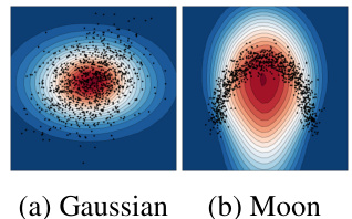
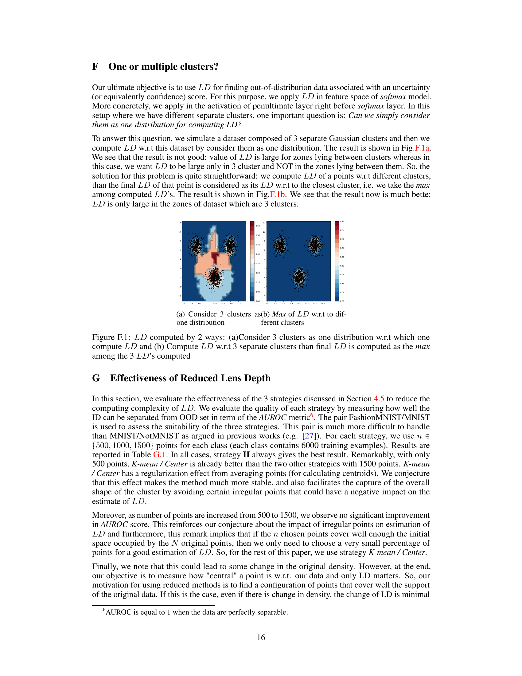
This figure shows a comparison of Lens Depth (LD) calculations using Euclidean distance for two different data distributions: a Gaussian distribution and a two-moons distribution. The contour lines represent the LD values, with darker shades indicating higher depth. The black points represent the data points themselves. The figure highlights that using Euclidean distance fails to properly capture the shape and density of the two-moons distribution, as the contour lines do not accurately reflect the cluster structure. In contrast, the Euclidean distance works relatively well for the Gaussian data because of the data’s spherical shape.

This figure visualizes the Fermat paths between two randomly selected points within a dataset for various values of the parameter α. The Fermat distance, a key component of the proposed method, is used to measure the distance between these points, taking into account the density and geometry of the data distribution. In panel (a), where α = 1, the Fermat path is a straight line representing the Euclidean distance. As α increases (b-d), the Fermat path starts to bend and adapts to the shape and density of the cluster. This demonstrates how the parameter α controls the sensitivity of the Fermat distance to the data’s underlying structure, which is essential in effectively capturing the depth of a point with respect to the data distribution.

This figure shows the results of applying Lens Depth (LD) with the sample Fermat distance on two datasets: moon and spiral. Subfigures (a) and (b) demonstrate the artifacts produced by using the classical Fermat distance, showing zones of constant LD values. In contrast, subfigures (c) and (d) illustrate the improved performance of the modified sample Fermat distance introduced by the authors, which accurately captures the distribution of both datasets.

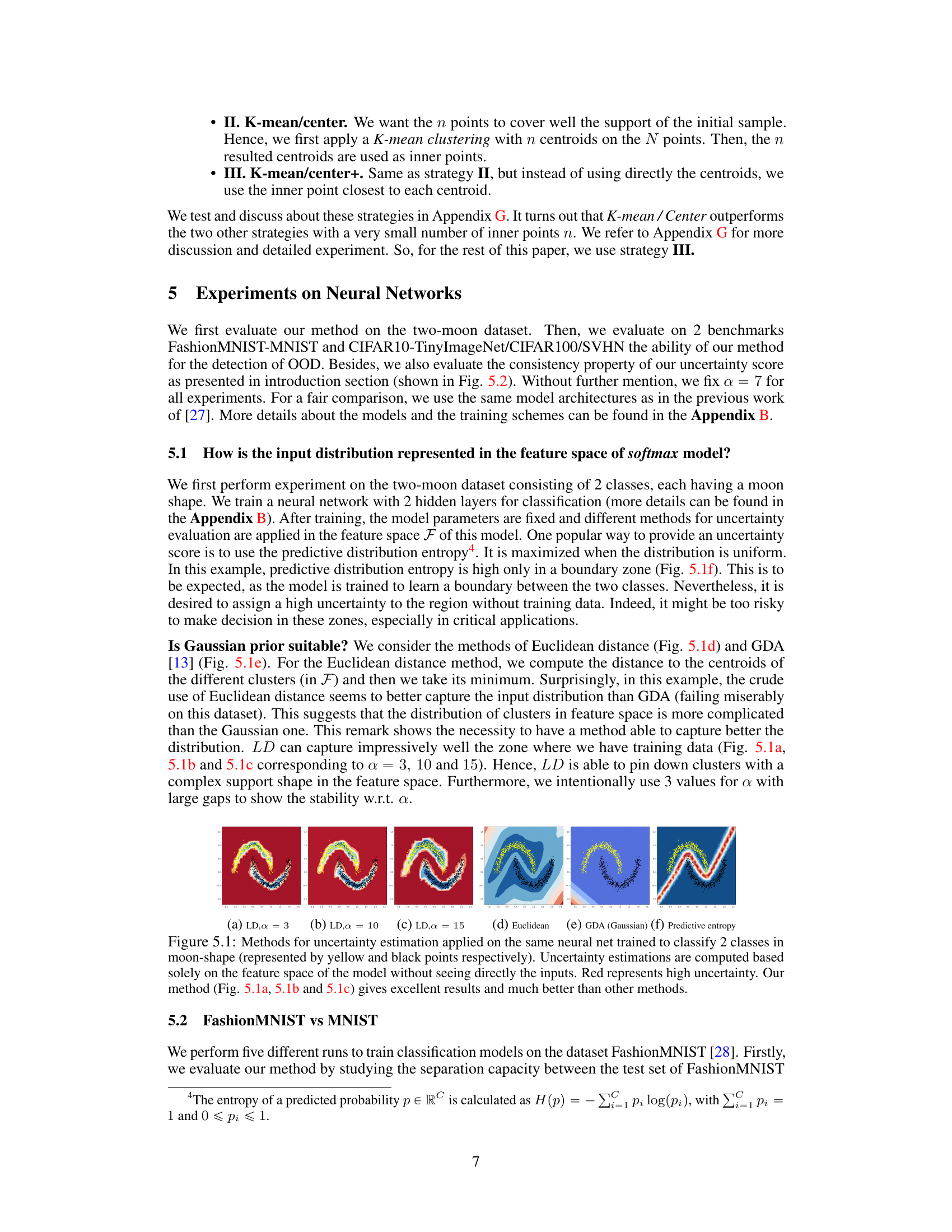
The figure shows a comparison of different uncertainty estimation methods applied to a two-moon dataset. The methods compared are Lens Depth (LD) with different values of the hyperparameter ‘a’, Euclidean distance, Gaussian Discriminant Analysis (GDA), and predictive entropy. The figure demonstrates that LD is able to capture the shape and density of the data distribution more effectively than the other methods, especially in complex shapes where GDA fails.

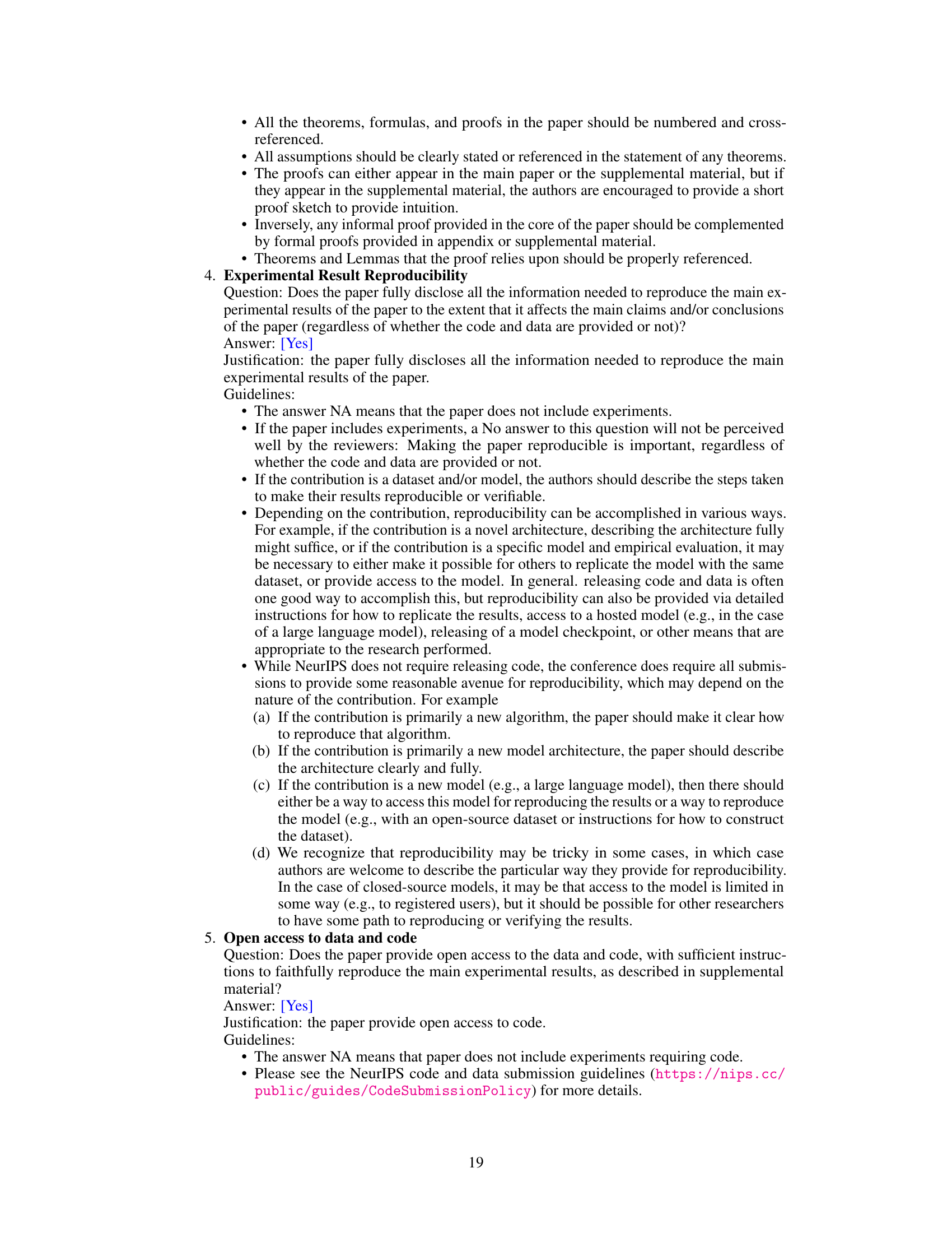
This figure shows the consistency curves for four different pairs of datasets: FashionMNIST/MNIST, CIFAR10/SVHN, CIFAR10/CIFAR100, and CIFAR10/Tiny-ImageNet. Each curve represents the accuracy of the model on the retained samples as a function of the percentage of samples rejected based on the Lens Depth (LD) score. The results are shown for 5 independent runs, with each curve corresponding to a separately trained model. The increasing trend of the curves demonstrates the effectiveness of LD as a measure of uncertainty; rejecting more uncertain samples (those with lower LD scores) increases the overall accuracy of the model on the remaining samples.

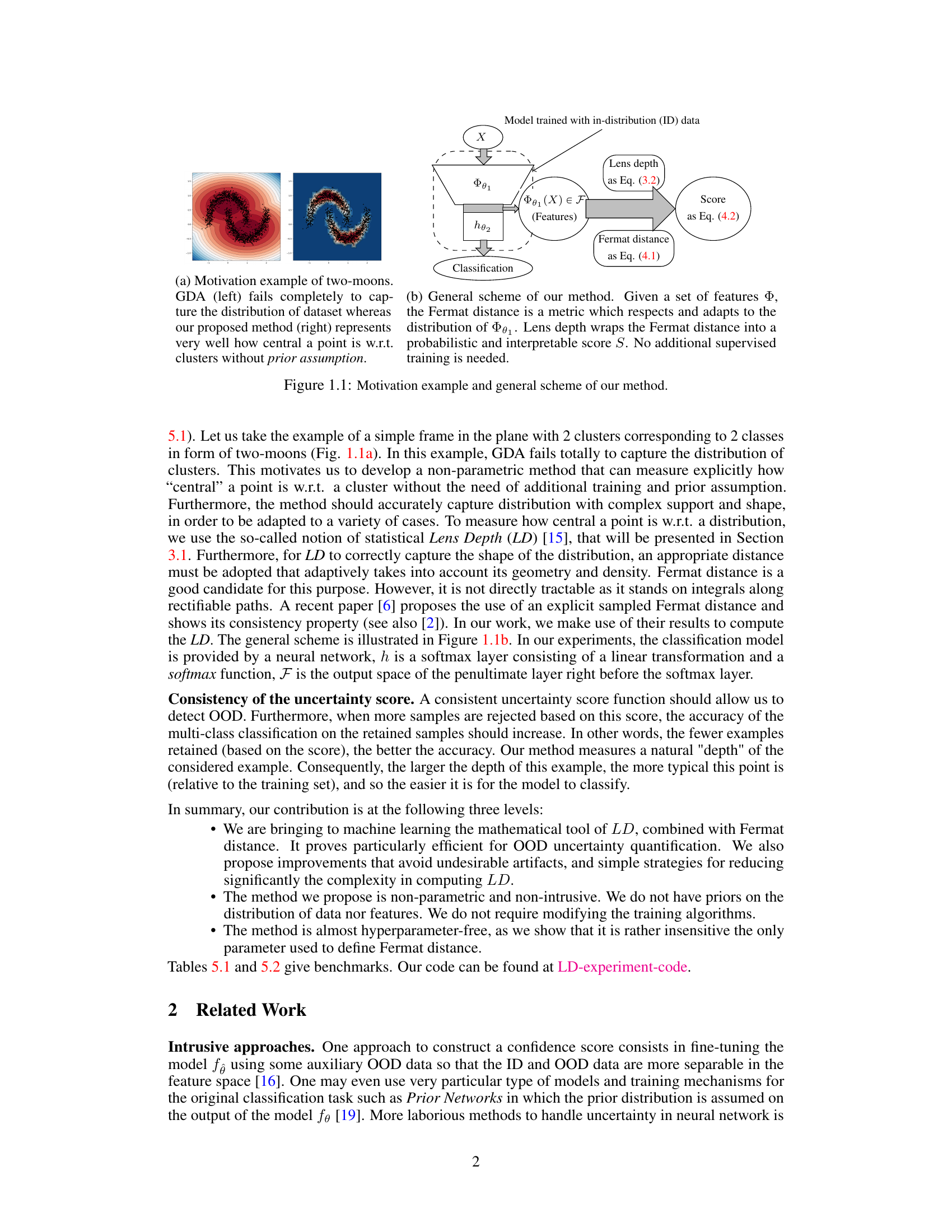
This figure shows the stability of the proposed method (LD with Sample Fermat Distance) when using only 20% of the data points from the spiral dataset. Ten independent trials were conducted, each using a different random subset of 200 points out of the original 1000. The contours of the LD level sets vary slightly across trials, demonstrating a degree of robustness, but the overall shape and structure of the distribution are consistently well-captured.
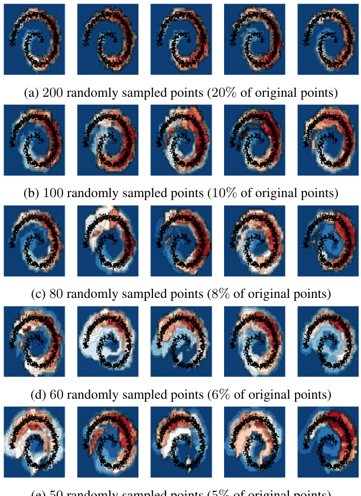
This figure shows the results of an experiment where the number of points used to compute the Lens Depth (LD) on a spiral dataset is progressively reduced. Each row shows results for a different percentage of the original 1000 data points (20%, 10%, 8%, 6%, 5%). The images illustrate that while LD can effectively capture the shape of the distribution with 20% of the data, its performance deteriorates as the data sparsity increases. At around 5-6% of the original data, LD loses the capacity to accurately represent the data distribution.

This figure shows the results of applying Lens Depth (LD) with the Sample Fermat Distance on two datasets: the two-moons dataset and the spiral dataset. The left two subfigures (a and b) show the results obtained using the original Sample Fermat Distance, which produces artifacts in the form of regions with constant LD values. The right two subfigures (c and d) show the results obtained using a modified version of the Sample Fermat Distance, which successfully captures the distributions.

This figure displays the consistency curves obtained from five independent runs for four different dataset pairs (FashionMNIST/MNIST, CIFAR10/SVHN, CIFAR10/CIFAR100, and CIFAR10/Tiny-ImageNet). Each curve shows the relationship between the percentage of samples rejected based on their Lens Depth (LD) score and the accuracy on the retained samples. The consistently increasing nature of the curves demonstrates that LD serves as a reliable indicator of uncertainty in model predictions, with higher accuracy observed as more uncertain samples are removed.
More on tables
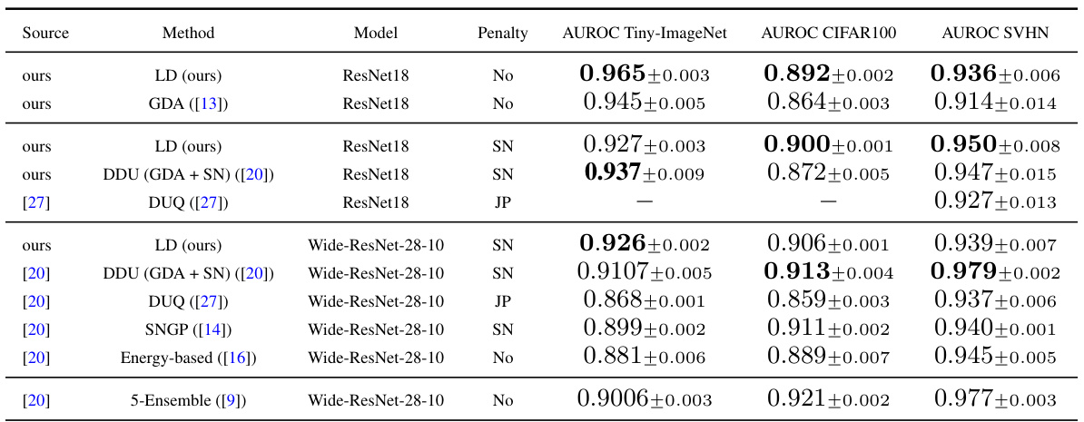
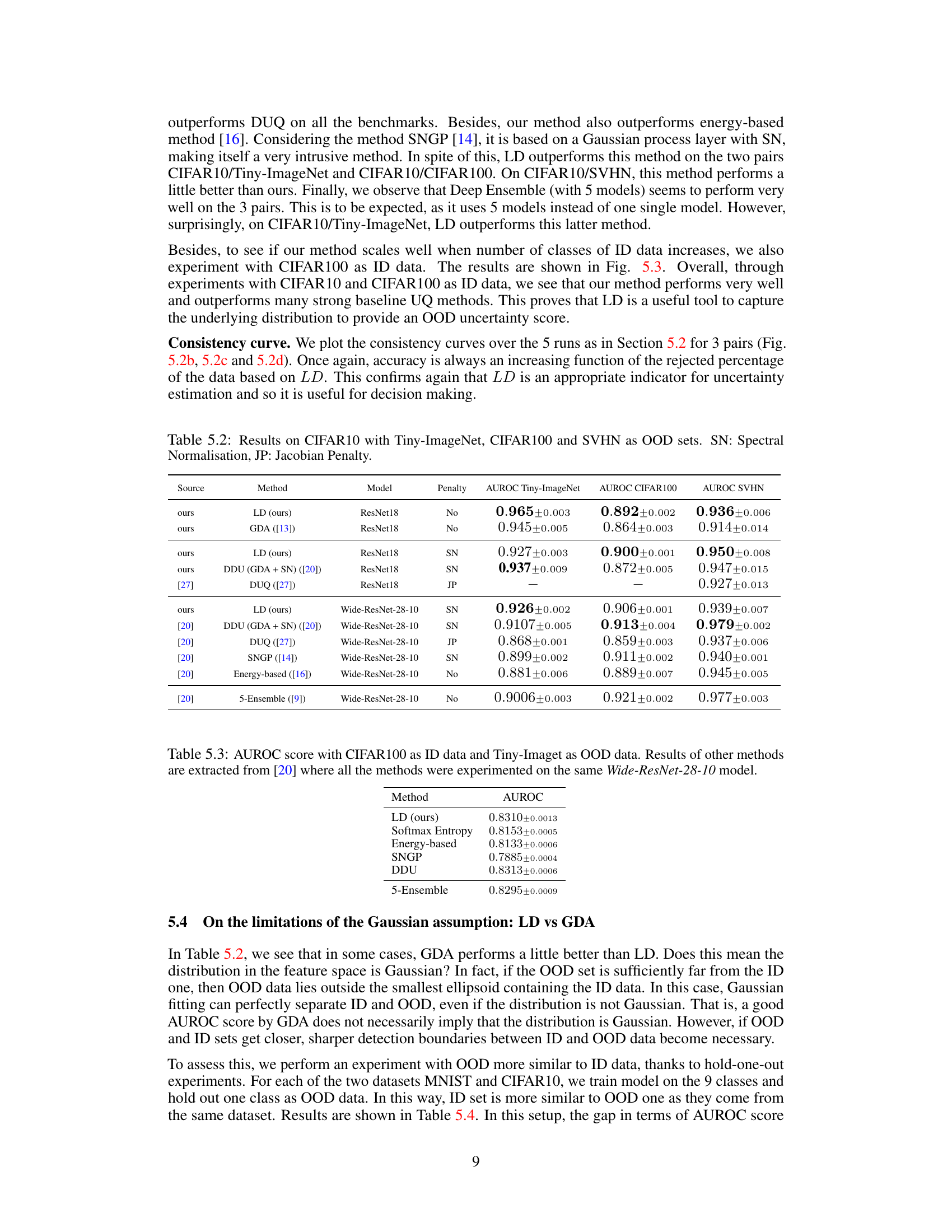
This table presents the AUROC scores achieved by different uncertainty quantification methods on the CIFAR10 dataset, using Tiny-ImageNet, CIFAR100, and SVHN as out-of-distribution (OOD) datasets. The methods compared include the proposed Lens Depth (LD) method, along with several baselines such as GDA, DDU, DUQ, SNGP, Energy-based, and Deep Ensembles. Different model architectures (ResNet18 and Wide-ResNet-28-10) and training penalties (SN and JP) are also considered. The table highlights the performance of LD against established techniques for OOD detection.

This table presents the AUROC (Area Under the Receiver Operating Characteristic curve) scores for out-of-distribution (OOD) detection experiments. The experiments used CIFAR-100 as the in-distribution (ID) dataset and Tiny-ImageNet as the out-of-distribution (OOD) dataset. The table compares the performance of the proposed Lens Depth (LD) method against several other state-of-the-art methods, including GDA, DUQ, SNGP, DDU, and an energy-based method. All methods were evaluated using the same Wide-ResNet-28-10 model for fair comparison. The results highlight the competitive performance of the LD method in this challenging OOD detection scenario.

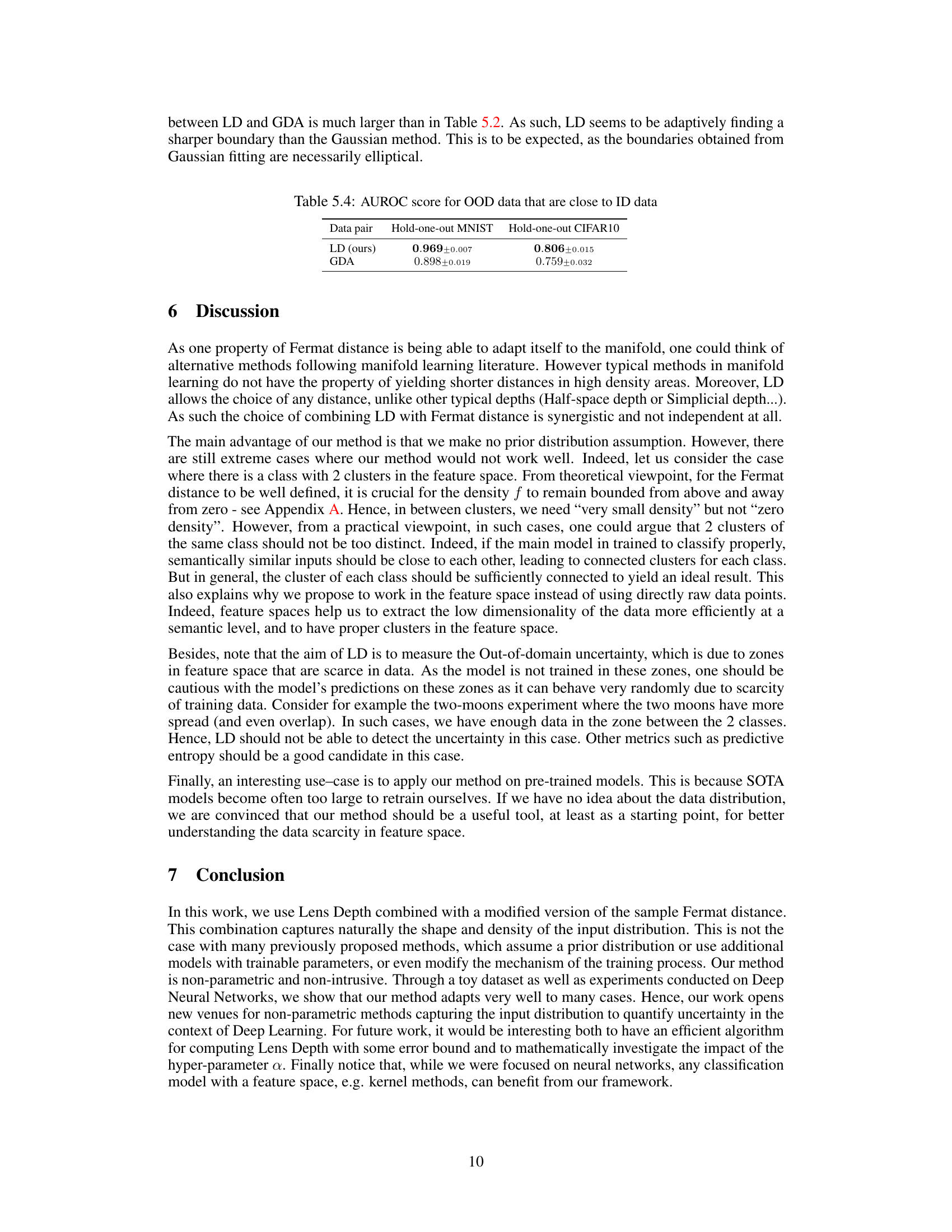
This table presents the Area Under the Receiver Operating Characteristic curve (AUROC) scores for out-of-distribution (OOD) detection. It compares the performance of the proposed Lens Depth (LD) method and the Gaussian Discriminant Analysis (GDA) method. The key difference here is that the OOD data is very similar to the in-distribution (ID) data, obtained by performing a hold-one-out experiment on both MNIST and CIFAR10 datasets. This setup highlights the ability of LD to effectively separate data with similar features compared to the GDA method which uses a Gaussian assumption.

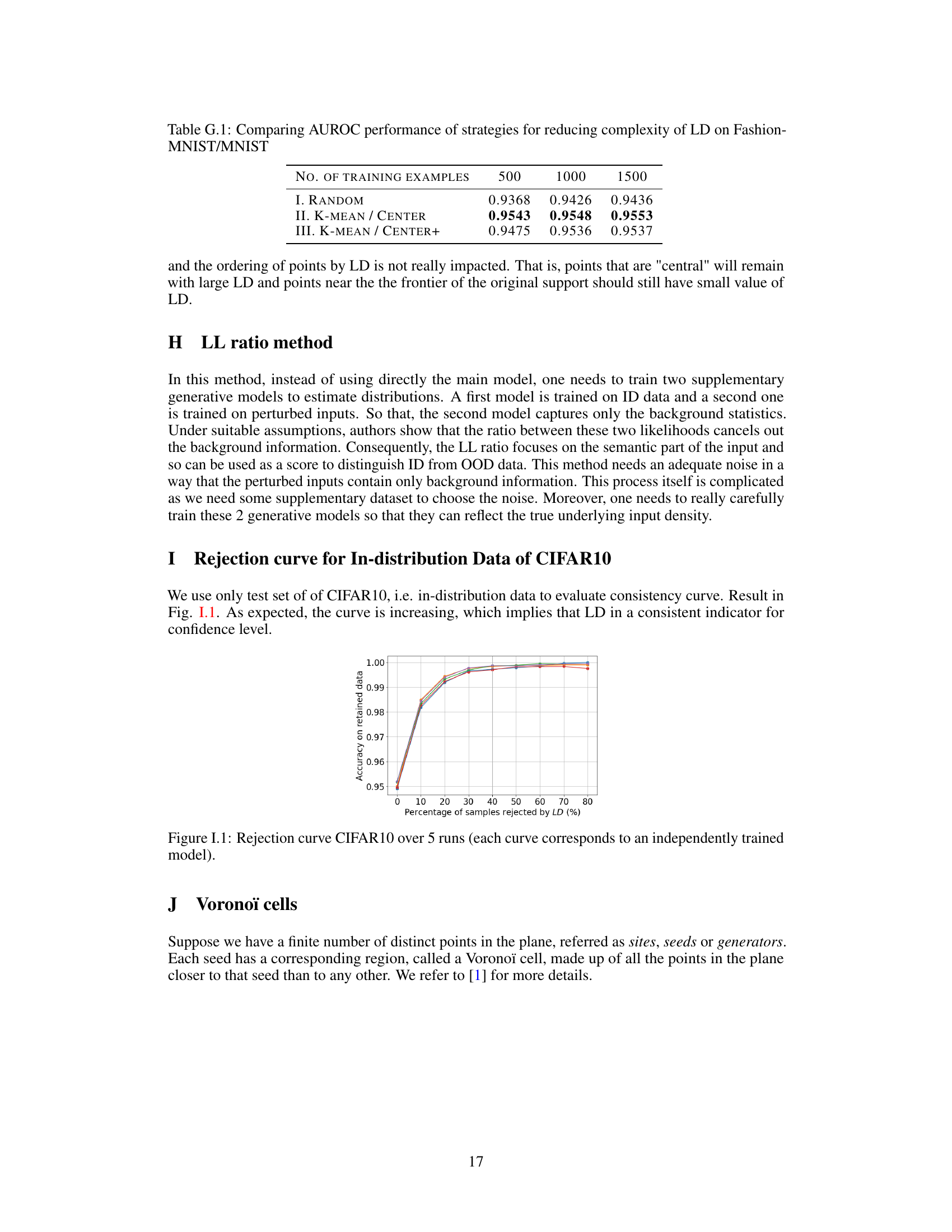
This table presents the Area Under the Receiver Operating Characteristic curve (AUROC) scores achieved by three different strategies to reduce the computational cost of Lens Depth (LD) in out-of-distribution (OOD) detection using the Fashion-MNIST dataset. The three strategies are: I. Random, II. K-Mean/Center, and III. K-Mean/Center+. Each strategy uses a varying number of training examples (500, 1000, and 1500) to compute the LD. The AUROC is a measure of the classifier’s ability to distinguish between in-distribution and out-of-distribution samples. Higher AUROC values indicate better performance. The table shows the AUROC for each strategy and the number of training examples used.
Full paper#
