↗ OpenReview ↗ NeurIPS Homepage ↗ Chat
TL;DR#
Many AI agents benefit from integrating planning into their learning process, but existing tree-based search methods often struggle with scalability due to their sequential nature. This paper introduces SPO, a model-based reinforcement learning algorithm that uses a parallelisable Monte Carlo approach to overcome these challenges. It allows for planning in both discrete and continuous action spaces without modifications.
SPO is grounded in the Expectation Maximisation (EM) framework and demonstrates statistically significant improvements in performance over model-free and model-based baselines in various experiments. Its parallel architecture enables efficient use of hardware accelerators, resulting in favorable scaling behavior. These improvements are shown both during training and inference.
Key Takeaways#
Why does it matter?#
This paper is important because it presents SPO, a novel and scalable model-based reinforcement learning algorithm that addresses the limitations of existing planning methods. Its parallelisable nature and applicability to both discrete and continuous action spaces make it highly relevant to current research in AI. The results suggest significant performance improvements across various benchmarks and open new avenues for research on efficient and scalable planning in RL.
Visual Insights#

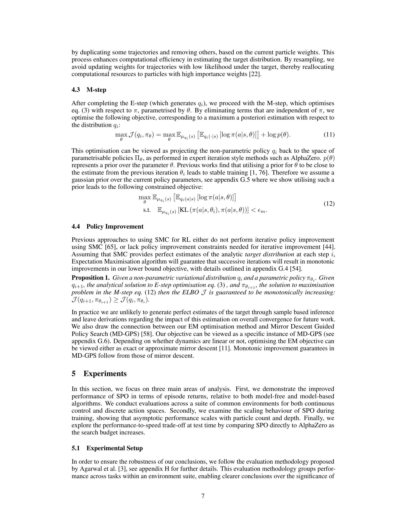
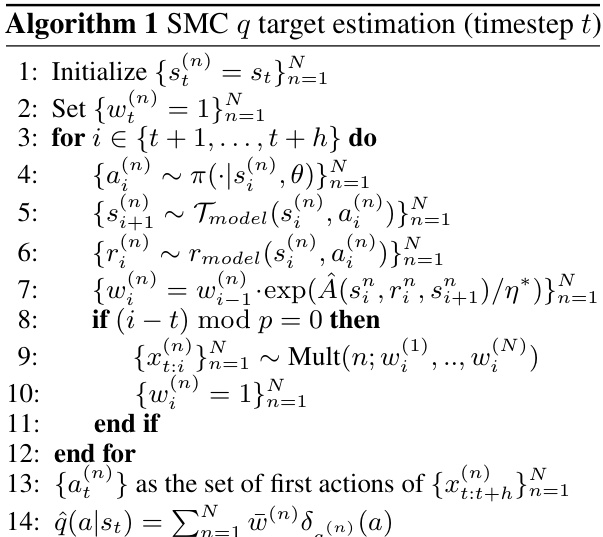
This figure illustrates the SPO search process, which consists of parallel rollouts and weight updates. Multiple trajectories are sampled according to the current policy (πi), and their importance weights are adjusted at each step, with periodic resampling to prevent weight degeneracy. The initial actions of the surviving particles after the search provides an estimate of the target distribution (qi), which is then used in the M-step (policy optimization).
This table lists the hyperparameters used for the SPO algorithm in both continuous and discrete environments. It details settings for various aspects of the algorithm, including learning rates, buffer sizes, batch sizes, rollout lengths, and exploration parameters, showing how these parameters were tuned differently based on the environment type.
In-depth insights#
SPO: Planning via EM#
The heading “SPO: Planning via EM” suggests a novel approach to reinforcement learning (RL) that integrates planning with the Expectation-Maximization (EM) algorithm. SPO likely leverages the power of EM for iterative policy improvement, alternating between an expectation step (E-step) to estimate a target distribution and a maximization step (M-step) to improve the policy. The E-step might involve Monte Carlo methods for efficient exploration of the state-action space, enabling planning in high-dimensional or continuous action settings. The EM framework provides a principled way to balance exploration and exploitation, guiding the search towards optimal policies. A key strength could be the algorithm’s inherent parallelizability, potentially enabling significant speed improvements via hardware acceleration. However, the success depends critically on the accuracy of the target distribution estimation during the E-step, and the effectiveness of the policy representation in the M-step. The practical challenges could involve managing computational cost associated with large sample sizes and the sensitivity to hyperparameter tuning. The overall effectiveness would depend heavily on the chosen Monte Carlo method, the chosen policy representation, and the efficiency of EM convergence.
SMC-based Policy Opt.#
A hypothetical ‘SMC-based Policy Opt.’ section would likely detail how Sequential Monte Carlo (SMC) methods are integrated into a policy optimization algorithm. SMC’s ability to sample from complex, high-dimensional probability distributions would be leveraged to efficiently explore the policy space. The core idea revolves around representing the policy as a probability distribution and using SMC to iteratively refine this distribution, moving towards an optimal policy. Key aspects would include the proposal distribution used for sampling, the importance weights assigned to samples, and a resampling scheme to prevent weight degeneracy. The algorithm might alternate between an E-step, where SMC estimates the distribution of optimal trajectories, and an M-step, where a new policy is learned based on the SMC estimates. This approach could offer advantages over traditional methods by enabling parallel computation and handling continuous action spaces more naturally. Convergence guarantees and computational efficiency compared to alternatives would also be critical elements of such a section, potentially highlighting the trade-offs between exploration and exploitation.
Parallel Scalability#
Achieving parallel scalability in reinforcement learning (RL) algorithms is crucial for tackling complex problems. The sequential nature of many planning algorithms, like Monte Carlo Tree Search (MCTS), often hinders scalability. Model-free approaches, while parallelizable to some extent, generally struggle to incorporate the planning component effectively. Model-based methods, especially those leveraging sampling-based planning like the Sequential Monte Carlo (SMC) methods explored in the paper, offer an attractive route to parallelism. By enabling independent evaluation of multiple actions or trajectories simultaneously, SMC-based approaches dramatically reduce the overall runtime, particularly beneficial when utilizing hardware accelerators. Effective parallelisation, however, requires careful consideration of the algorithm’s design, ensuring that the computational workload is evenly distributed, and that communication overhead between parallel processes remains minimal. The paper demonstrates that integrating SMC within the Expectation Maximization (EM) framework is a promising approach to attain robust policy improvement while harnessing the advantages of parallel processing.
Empirical Evaluation#
A robust empirical evaluation section is crucial for validating the claims of any research paper. It should present a comprehensive set of experiments designed to thoroughly test the proposed method’s performance and generalizability. Methodologically sound experiments, employing appropriate baselines and statistical analysis, are essential. Clear descriptions of experimental setups, hyperparameters, and evaluation metrics are necessary for reproducibility. Visualization of results using graphs and tables helps to convey findings effectively, particularly when comparing different approaches. The discussion should go beyond simple observations, providing thoughtful analysis of the results and relating them back to the paper’s main claims. Addressing potential limitations and suggesting avenues for future work further enhances the section’s value. Overall, a strong empirical evaluation section instills confidence in the research’s validity and its potential impact.
Future Research#
Future research directions stemming from this Sequential Monte Carlo Policy Optimization (SPO) paper could involve several key areas. Improving the SMC algorithm itself is paramount; exploring alternative proposal distributions or resampling strategies could enhance efficiency and accuracy, especially in high-dimensional or stochastic environments. Investigating learned world models instead of perfect simulators would greatly expand the applicability of SPO to real-world scenarios. Adapting SPO for stochastic environments presents another significant challenge, requiring careful consideration of importance weight updates and exploration strategies. Finally, a thorough exploration of the hyperparameter sensitivity and impact on performance across diverse problem settings, including careful analysis of KL regularization and exploration techniques, would prove valuable. Combining theoretical analysis with extensive empirical validation across a broader range of benchmarks is crucial to fully realize SPO’s potential.
More visual insights#
More on figures

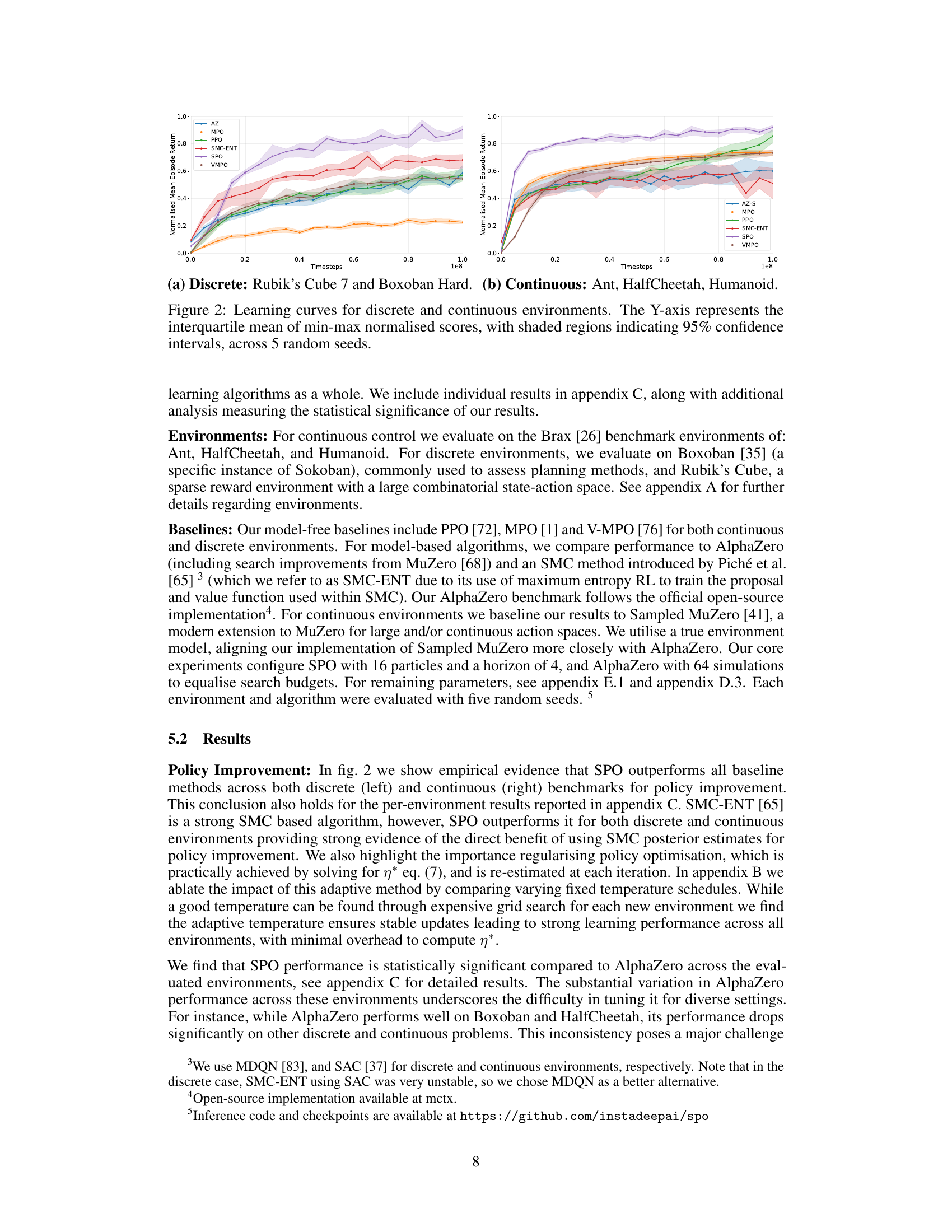
This figure displays the learning curves for both discrete and continuous control tasks. The y-axis shows the normalized mean episode return, representing the average performance of each algorithm across 5 different random seeds. Shaded regions show 95% confidence intervals, illustrating the variability in performance. The x-axis represents the number of timesteps during training. The figure compares SPO’s performance against several baselines (MPO, PPO, VMPO, SMC-ENT, AlphaZero) across various environments (Ant, HalfCheetah, Humanoid, Rubik’s Cube 7, Boxoban Hard). The results highlight SPO’s improved and more consistent performance across diverse tasks compared to other methods.

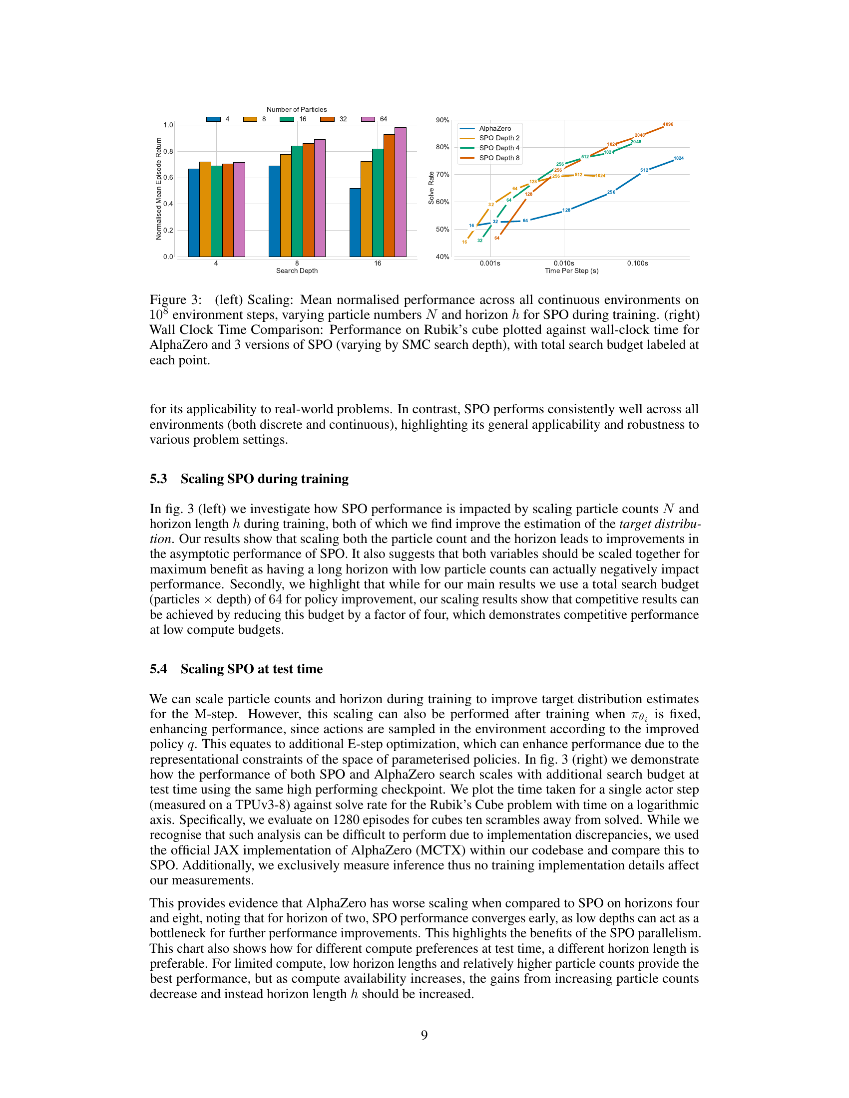
This figure shows two plots. The left plot shows how the performance of SPO scales with the number of particles and the search depth (horizon) during training. The x-axis represents search depth (horizon), and the y-axis shows the normalized mean episode return. Different colored bars show results for different numbers of particles. The right plot compares the wall-clock time performance of AlphaZero and SPO on the Rubik’s Cube task. The x-axis represents time per step, and the y-axis shows the solve rate. Different colored lines represent different versions of SPO with varying search depths (horizons). The total search budget for each point is also shown.

This figure illustrates the SPO search process. Multiple trajectory samples (particles) are generated in parallel using the current policy. At each step, particle weights are updated based on their performance, favoring high-performing trajectories. Periodically, particles are resampled to focus computation on the most promising trajectories. The initial actions of the surviving particles provide an estimate of the target distribution, used to improve the policy in the M-step of the EM algorithm.

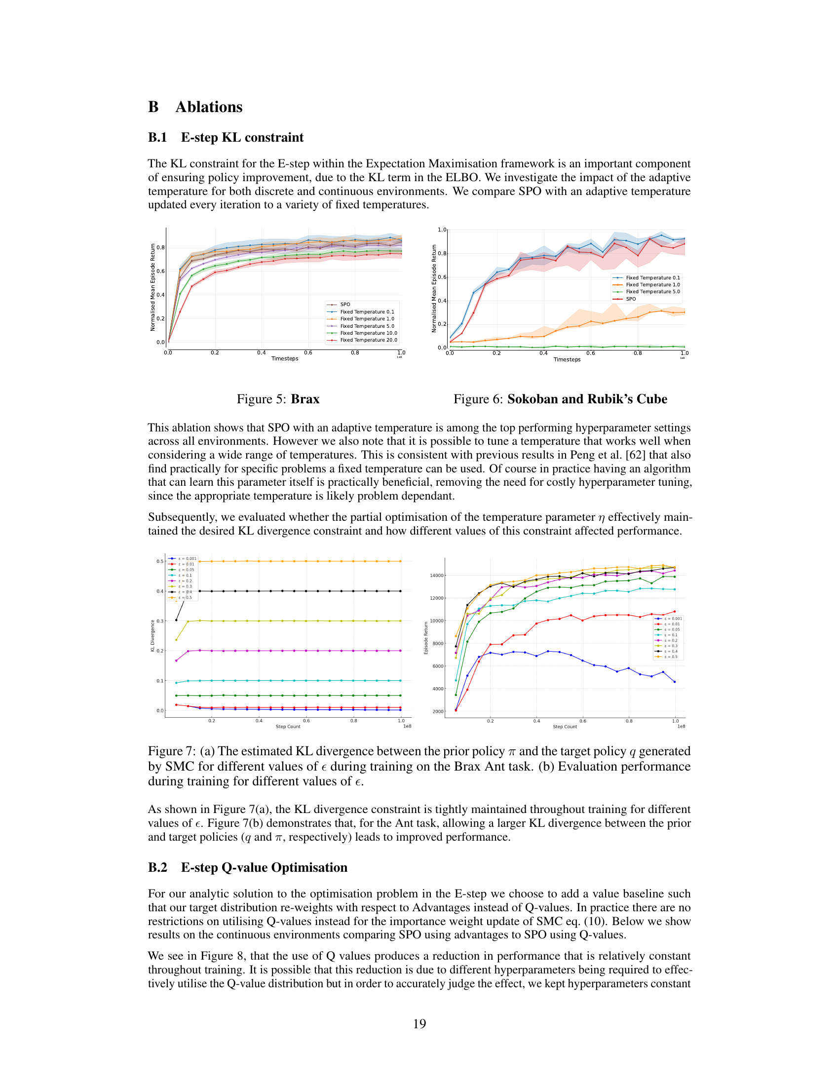
This ablation shows that SPO with an adaptive temperature is among the top performing hyperparameter settings across all environments. However we also note that it is possible to tune a temperature that works well when considering a wide range of temperatures. This is consistent with previous results in Peng et al. [62] that also find practically for specific problems a fixed temperature can be used. Of course in practice having an algorithm that can learn this parameter itself is practically beneficial, removing the need for costly hyperparameter tuning, since the appropriate temperature is likely problem dependant. Subsequently, we evaluated whether the partial optimisation of the temperature parameter η effectively maintained the desired KL divergence constraint and how different values of this constraint affected performance.
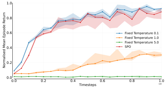
This figure shows the ablation study on the effect of using fixed temperature values for the KL divergence constraint in the Expectation Maximisation framework against using an adaptive temperature updated every iteration in SPO. The x-axis represents training timesteps, while the y-axis represents the normalised mean episode return. The plot compares SPO with an adaptive temperature to SPO with fixed temperature values of 0.1, 1.0, 5.0, and 10.0. The shaded regions represent 95% confidence intervals. The results suggest that using an adaptive temperature leads to better performance overall compared to using various fixed temperatures.
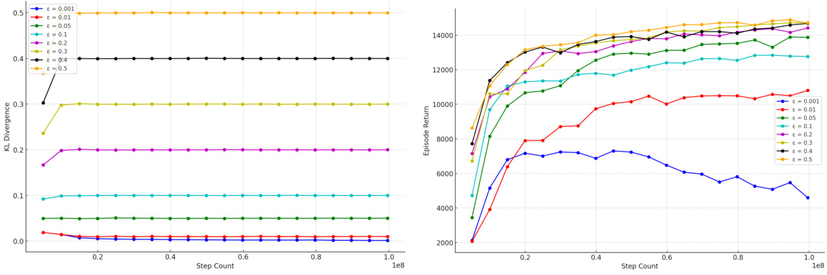
This figure shows the effect of different KL divergence constraints (ε) on both the KL divergence between the prior and target policies and the resulting performance. Subfigure (a) plots the KL divergence over training steps for various ε values, demonstrating how the constraint is maintained. Subfigure (b) shows the corresponding performance curves, indicating that a larger KL divergence can lead to better performance.

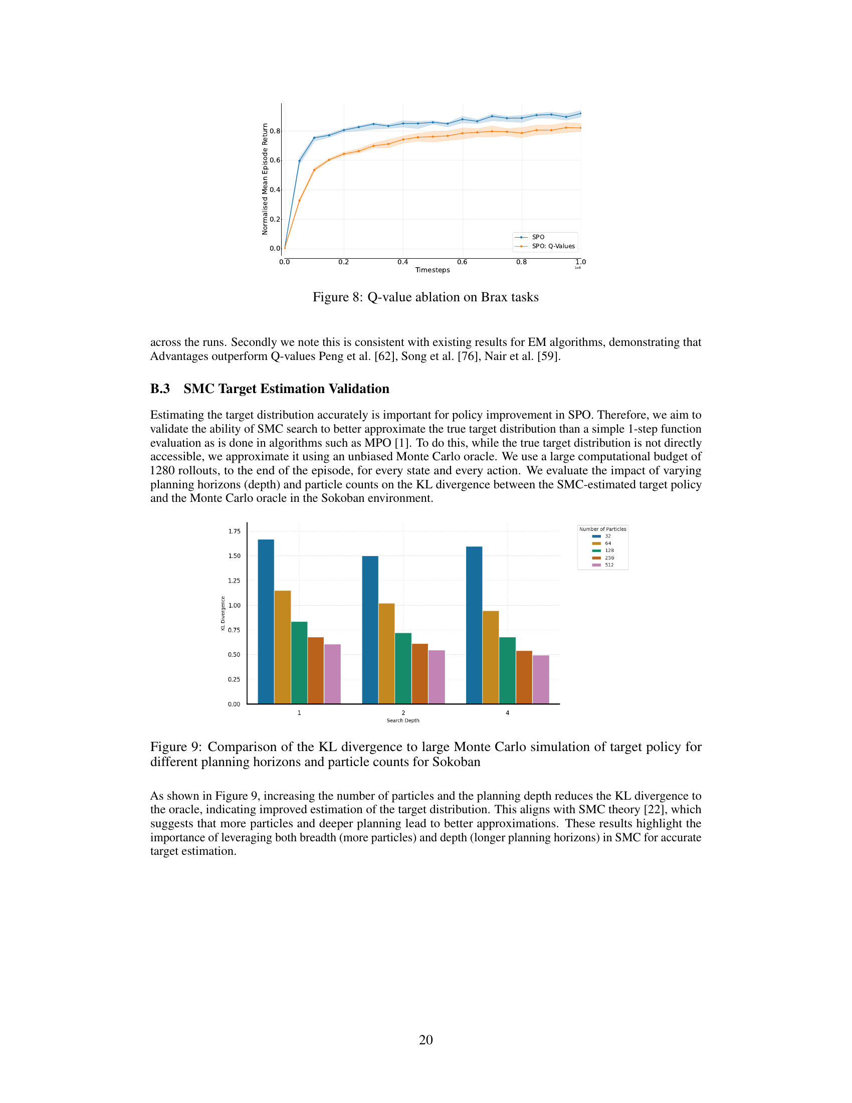
This ablation study compares the performance of SPO using advantages against using Q-values for the policy improvement step within the Expectation Maximisation framework. The results show that using advantages consistently outperforms using Q-values across all Brax benchmark tasks. The shaded areas represent 95% confidence intervals across five random seeds.
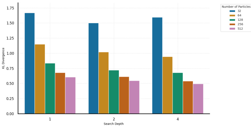
This figure shows the KL divergence between the SMC estimated target policy and a Monte Carlo oracle for Sokoban. It demonstrates the impact of increasing the number of particles and planning depth (horizon) on the accuracy of the SMC estimation. Higher particle counts and deeper planning horizons lead to lower KL divergence, indicating improved estimation of the target distribution. The results highlight the importance of balancing breadth (particles) and depth (planning horizon) in SMC for accurate target estimation.

This figure presents a comparison of different reinforcement learning algorithms across various continuous control tasks from the Brax suite. It shows the median, interquartile mean (IQM), and mean normalized episode returns achieved by each algorithm. The 95% confidence intervals reflect the uncertainty in the performance estimates due to the limited number of runs and random seeds. The results are aggregated and visualized across multiple tasks to give a robust comparison of the algorithms.

This figure shows the performance comparison across different algorithms on the Brax suite of continuous control environments. Three performance metrics are displayed: Median, Interquartile Mean (IQM), and Mean. Each metric represents the aggregated performance across all tasks and seeds within the Brax environment. The error bars represent the 95% confidence intervals, calculated using stratified bootstrapping, providing a measure of the statistical uncertainty associated with the performance estimates.
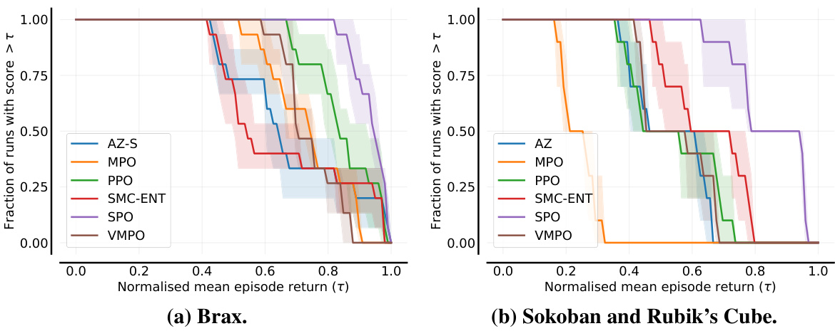
This figure presents performance profiles which visually illustrate the distribution of scores across all tasks and seeds for each algorithm. The Y-axis shows the fraction of runs achieving a normalized score greater than the value on the X-axis. The shaded areas represent 95% confidence intervals, obtained through stratified bootstrapping. This visualization helps to compare the algorithms’ performance across a range of score thresholds and highlights the consistency (low variance) of the algorithms. The curves’ relative positions indicate the algorithms’ relative performance.

This figure presents the probability of improvement plots for both Brax and Sokoban/Rubik’s Cube environments. It visually shows the likelihood that SPO outperforms another algorithm (VMPO, SMC-ENT, AZ, PPO, MPO) on a randomly selected task. The plots show that SPO has a high probability of improvement compared to all baselines, with all probabilities exceeding 0.5 and their confidence intervals (CIs) entirely above 0.5. This indicates statistical significance according to the methodology used in the paper.

This figure presents the performance of different reinforcement learning algorithms across various continuous and discrete control environments. Each subplot corresponds to a specific environment (Ant, HalfCheetah, Humanoid, Sokoban, and Rubik’s Cube). The y-axis shows the mean episode return, a metric measuring the average reward accumulated during an episode. The x-axis represents the training progress, measured in timesteps. The shaded regions indicate 95% confidence intervals, highlighting the uncertainty associated with the results. The results illustrate that SPO consistently outperforms other algorithms across multiple environments.
More on tables

This table presents the dataset sizes for different difficulty levels in the Boxoban dataset used in the paper’s experiments. It shows the number of levels available for training, validation, and testing, as well as separate counts for ‘Medium’ and ‘Hard’ difficulty levels. This breakdown is important because the paper evaluates performance on specific subsets of the dataset (e.g., the ‘Hard’ dataset) to assess the algorithms’ capabilities in more challenging scenarios.

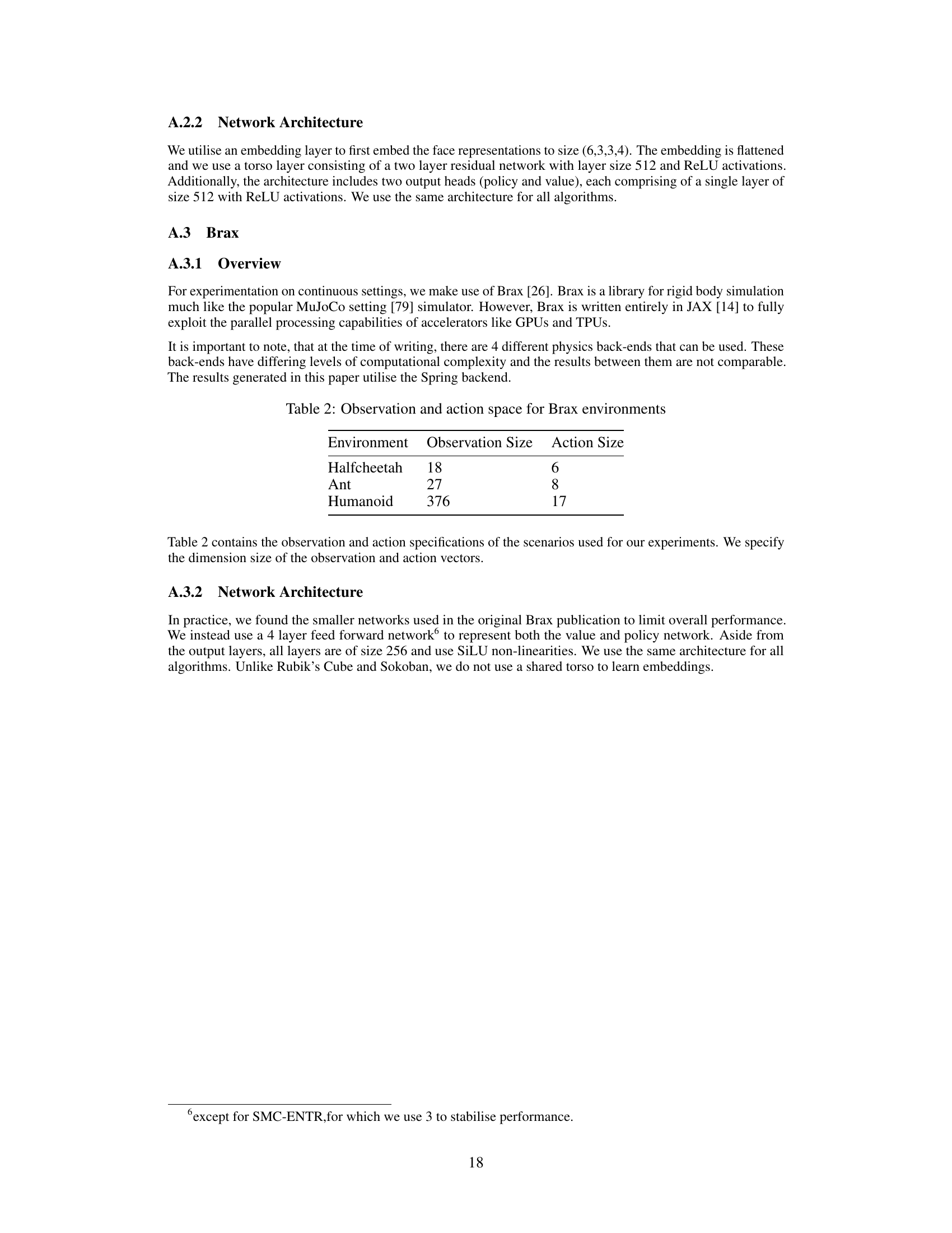
This table shows the observation and action space sizes for three different Brax environments: Halfcheetah, Ant, and Humanoid. The observation size refers to the dimensionality of the state representation provided to the reinforcement learning agent, while the action size corresponds to the number of dimensions in the action space that the agent can choose from.
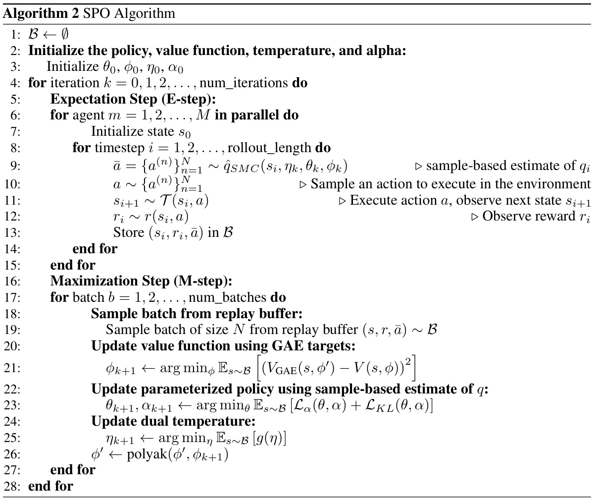
This table lists the hyperparameters used in the SPO algorithm for both continuous and discrete environments. It breaks down the settings for various aspects of the algorithm, including learning rates, buffer sizes, batch sizes, rollout lengths, and exploration parameters. The values specified are those found to work well in experiments. The table helps to clarify the specific configurations used during the training and evaluation processes reported in the paper.
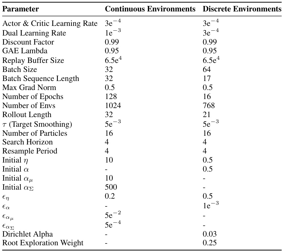
This table lists the hyperparameters used for the SPO algorithm in both continuous and discrete environments. It details settings for learning rates (actor, critic, and dual), discount factor, GAE lambda, replay buffer size, batch size, batch sequence length, maximum gradient norm, number of epochs, number of environments, rollout length, target smoothing, number of particles, search horizon, resample period, initial values for temperature (η), exploration (α), and KL divergence constraints (ε), and other parameters such as Dirichlet Alpha and root exploration weight.
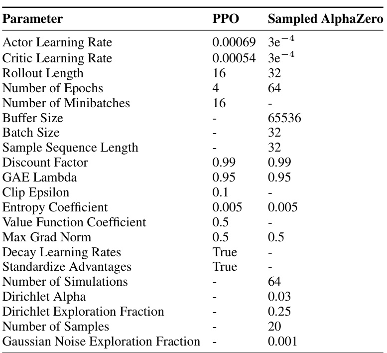
This table lists the hyperparameters used for training both PPO and Sampled AlphaZero, highlighting the differences in their configurations for continuous control tasks. It covers various aspects of the training process, including learning rates, rollout lengths, batch sizes, discount factors, and exploration strategies.

This table lists the hyperparameters used for training the MPO and VMPO algorithms in the paper. It shows various parameters, including rollout length, number of epochs, buffer size, batch size, sample sequence length, learning rates (actor and critic), target smoothing, discount factor, maximum gradient norm, and whether learning rates decay. Additionally, parameters specific to MPO and VMPO such as the initial values of the temperature and exploration parameters are shown.

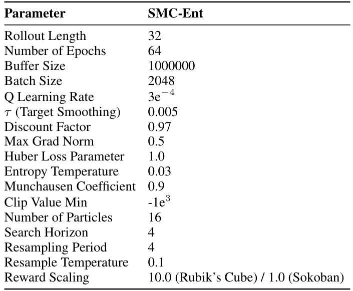
This table lists the hyperparameters used for the SMC-Ent baseline algorithm in the paper’s experiments. It includes parameters related to training, the SMC algorithm itself, and the Q-learning used within the algorithm. The hyperparameters are specific to the SMC-Ent algorithm and were used for comparison with the proposed SPO method in the experiments.
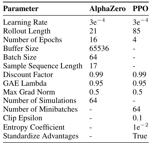
This table lists the hyperparameters used for the AlphaZero and PPO algorithms in the paper’s experiments. It includes settings for learning rates, rollout lengths, the number of epochs, buffer and batch sizes, sample sequence length, discount factor, GAE lambda, max grad norm, number of simulations (AlphaZero only), number of minibatches (PPO only), clip epsilon (PPO only), entropy coefficient (PPO only), and whether or not advantages are standardized (PPO only). These hyperparameters were crucial in configuring the algorithms for the experiments, especially in controlling the balance between exploration and exploitation.

This table lists the hyperparameters used for training the MPO and VMPO baseline algorithms in the paper. It provides a detailed comparison of the settings used for both algorithms, highlighting differences in parameters such as learning rates, rollout length, batch size, and other key optimization parameters.
This table lists the hyperparameters used for the SPO algorithm in both continuous and discrete environments. It includes settings for learning rates, discount factors, buffer sizes, batch sizes, rollout lengths, and other parameters crucial for model training and performance.

This table compares several Expectation-Maximization (EM) based reinforcement learning algorithms. It highlights key differences in their E-step (expectation step) and M-step (maximization step) optimization objectives (G), whether trust regions are used in these steps, the method used for estimating the G objective, and the depth and breadth of the search process used by each algorithm. The table shows that different algorithms take different approaches to planning, including using analytic solutions, temporal difference (TD) learning, Monte Carlo Tree Search (MCTS), or Sequential Monte Carlo (SMC).

This table lists the hyperparameters used for training both the Proximal Policy Optimization (PPO) and Sampled AlphaZero algorithms. It provides a detailed comparison of the settings used for each algorithm across various parameters such as learning rates, rollout length, batch size, discount factor, and more. This allows for a clear understanding of the differences in training configurations used for both methods.

This table lists the hyperparameters used in the SPO algorithm for both continuous and discrete environments. It specifies values for parameters related to the actor and critic networks (learning rates, discount factor), the value function update (GAE lambda), replay buffer and batch sizes, gradient clipping, training epochs, and the number of environments used during training. It also shows hyperparameters specific to the SPO method, including the number of particles, search horizon, resampling period, initial values for the temperature parameter (η), alpha (α), and exploration weight. Finally, hyperparameters for discrete environments (Dirichlet alpha and root exploration weights) are also detailed.
Full paper#
