High-probability complexity bounds for stochastic non-convex minimax optimization

↗ OpenReview ↗ NeurIPS Homepage ↗ Chat

TL;DR

#

Key Takeaways

#

Why does it matter?

#

This paper is crucial for researchers working on nonconvex minimax problems, a common challenge in machine learning. It provides the first high-probability complexity guarantees for solving such problems using a single-loop method, addressing a major gap in the field. This opens avenues for developing more robust and efficient algorithms with stronger theoretical foundations. The results are especially relevant for applications like GAN training and distributionally robust optimization, where high-probability bounds are crucial for reliable performance.

Visual Insights

#

This figure shows the results of applying the smoothed alternating gradient descent ascent (sm-AGDA) algorithm to a nonconvex-PL (NCPL) minimax problem. The left panel displays the average of the stationarity measure Mk(t) across 25 sample paths, plotted against the number of iterations. The right panel shows the average squared distance I(t) to the solution across the same 25 sample paths. In both panels, the shaded regions represent the range of values obtained across all 25 sample paths, highlighting the variability of the results. The two different line colors represent the results obtained with different step sizes (τ₁ = 2 and τ₁ = 120). The figure demonstrates the algorithm’s convergence behavior and the effect of step size on convergence speed and variability.

This table summarizes existing high-probability complexity bounds from the literature for various minimax optimization problems and compares them to the new results obtained in this paper. It shows the complexity (number of stochastic gradient calls) needed to achieve a certain level of stationarity (defined by different metrics) with a specified probability for different problem classes (convex-concave, monotone variational inequality, and nonconvex-PL). The table highlights whether each method allows for nonconvexity in the primal variable.

In-depth insights

#

NCPL Guarantees

#

The heading ‘NCPL Guarantees’ likely refers to the high-probability complexity guarantees established for Nonconvex-PL (NCPL) minimax problems. The core contribution is providing theoretical bounds on the number of iterations needed to reach an approximate stationary point with high probability. This is a significant advance because existing analyses often focus on expected values, which do not control for worst-case scenarios. The authors’ focus on the smoothed alternating gradient descent ascent (sm-AGDA) algorithm and the PL condition for the dual variable is key to the derivation of these bounds. The results are particularly impactful for machine learning applications, as many optimization problems involving GANs and adversarial learning fall into this category. Light-tailed assumptions on the stochastic gradients are crucial for establishing the high-probability guarantees. The work likely provides a novel Lyapunov function or concentration inequality to derive these bounds. Furthermore, empirical validation on synthetic and real-world problems should be included to demonstrate the practical relevance and tightness of the theoretical findings.

Sm-AGDA Analysis

#

The Sm-AGDA analysis section would likely delve into the theoretical underpinnings of the Smoothed Alternating Gradient Descent Ascent method. It would likely begin by formally defining the algorithm, outlining the key parameters and their impact on convergence. A crucial aspect would be the presentation of the algorithm’s convergence guarantees. High-probability bounds, particularly those under non-convex settings, would be a core focus, contrasting with standard expected value analyses. The analysis might involve constructing and analyzing a Lyapunov function to establish the descent properties of Sm-AGDA, demonstrating a decrease in the Lyapunov function value over iterations. Furthermore, the impact of light-tailed stochastic gradients on the method’s convergence would be examined, potentially leading to refined convergence rates. The section would also likely contain discussions of the algorithm’s computational complexity and the relationship between its convergence and the problem’s parameters like Lipschitz constants or the Polyak-Łojasiewicz (PL) condition. Finally, there could be a discussion on practical implementation details or considerations for efficiently deploying the method.

High-Prob. Bounds

#

The section on “High-Prob. Bounds” likely details high-probability complexity guarantees for nonconvex minimax optimization problems. It moves beyond expectation-based analyses, which only provide average-case convergence rates, to offer stronger claims about the algorithm’s performance with a specified probability. This is crucial for real-world applications where a guaranteed level of performance is needed, rather than just average performance. The focus is likely on establishing bounds on the number of iterations or stochastic gradient computations required to achieve a certain level of accuracy (e.g., finding an ε-stationary point) with probability at least 1-δ, where δ is a small probability of failure. The theoretical results would likely involve sophisticated concentration inequalities to handle the inherent randomness in stochastic gradient methods. The analysis likely considers assumptions about the smoothness and structure of the objective function, as well as the properties of the stochastic gradient noise. The authors might compare the high-probability bounds with existing expectation-based bounds, showcasing the benefits and potential costs of this stronger guarantee. Numerical experiments would validate the theory, possibly showing how the high-probability bounds translate into practical performance in different settings.

DRO Experiments

#

The section on “DRO Experiments” would ideally delve into the practical application of the research on distributionally robust optimization problems. It should showcase the efficacy of the proposed sm-AGDA algorithm on real-world datasets, comparing its performance against established baselines such as SAPD+ and SMDAVR. Key aspects to highlight include the choice of datasets, their characteristics (size, dimensionality, and noise levels), the specific DRO problem formulation used, and the hyperparameter tuning strategies employed. A detailed analysis of the results, potentially involving statistical significance tests to validate the findings and assess the impact of the high-probability guarantees, should be provided. Visualizations such as histograms and CDFs would strengthen the presentation of the experimental results, demonstrating the algorithm’s ability to achieve stationarity with high probability under various conditions. Finally, a discussion on the scalability and computational cost of the sm-AGDA algorithm in the context of the DRO experiments is crucial to demonstrate its practical viability. The overall goal should be to demonstrate that the theoretical contributions translate into tangible improvements in the performance of DRO solutions, showcasing the algorithm’s robustness and efficiency in solving challenging real-world optimization tasks.

Future Works

#

Future research could explore several promising avenues. Extending the high-probability guarantees to other nonconvex minimax settings beyond the PL condition is crucial. This includes investigating weaker assumptions on the objective function or exploring different algorithm classes. A key challenge is to develop tighter high-probability bounds, ideally removing the log(1/δ) factor from the current complexity. Investigating the impact of heavy-tailed noise on the algorithm’s performance and the development of robust methods is important. Furthermore, a deeper exploration into the practical aspects, including algorithm parameter tuning and scalability, warrants further study. Finally, exploring applications of the developed techniques in various machine learning tasks, such as GAN training and robust optimization, would provide valuable insights into real-world performance and impact.

More visual insights

#

More on figures

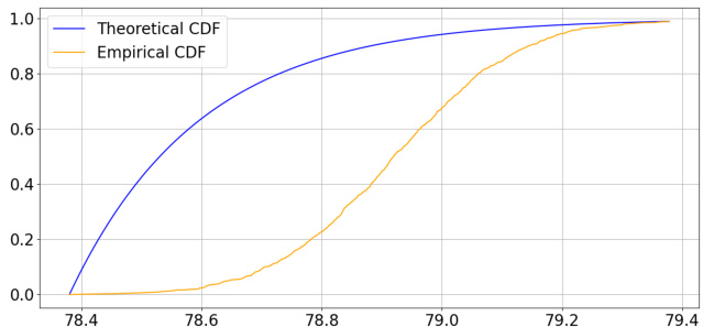
The figure compares the cumulative distribution function (CDF) of the theoretical upper bound on the stationarity measure from Theorem 11 with the empirical CDF obtained from 1000 sample paths of the sm-AGDA algorithm for Problem (13). The theoretical CDF provides an upper bound on the quantiles of the stationarity measure. The empirical CDF shows the actual distribution of the stationarity measure observed in the simulations. The plot shows that the theoretical bounds are reasonably tight, especially at higher quantiles. The difference between the two curves may be because the theoretical quantiles are designed to capture the worst-case behavior across the class of NCPL problems, while the specific NCPL example used in the simulations may not necessarily represent a worst-case scenario.

The figure displays the histograms of the stationarity measure (log10 ||f(xt,yt)||2) for three algorithms (sm-AGDA, SAPD+, and SMDAVR) across three datasets (a9a, gisette, and sido0). Each algorithm was run 200 times. The histograms show the distribution of the stationarity measure at two different points in the training process: after 20 epochs (first row) and at the end of training (second row). This visualization helps to compare the convergence behavior and the concentration of the stationarity measure for each algorithm.

Full paper

#