Hybrid Top-Down Global Causal Discovery with Local Search for Linear and Nonlinear Additive Noise Models

xnmm1jThkv

Sujai Hiremath et el.

TL;DR
#

Learning unique causal relationships from data is challenging. Existing methods either struggle with high dimensionality or rely on strong assumptions about the data. This makes it difficult to apply these methods to real-world problems with complex, high-dimensional data. Furthermore, many real-world systems exhibit nonlinear relationships, posing another challenge for causal discovery methods.

This paper introduces a new hybrid approach to tackle these challenges. The method uses a two-stage process. First, it employs a novel topological sorting algorithm that efficiently organizes the variables in the data based on their causal relationships. Then, it applies a constraint-based algorithm to identify and remove incorrect edges from the causal graph. This hybrid approach is effective for both linear and nonlinear data with arbitrary noise distributions, and significantly improves the accuracy and efficiency of causal discovery.

Key Takeaways
#

Why does it matter?
#

This paper is crucial for researchers in causal discovery because it presents a novel hybrid approach that tackles the limitations of existing methods. It offers theoretical guarantees and empirical validation, paving the way for more accurate and efficient causal inference in complex systems. Its focus on sparse graphs and nonlinear relationships addresses important challenges in high-dimensional applications.

Visual Insights
#

This figure shows a simple directed acyclic graph (DAG) with three nodes, illustrating different types of nodes and their relationships. Node x₁ is a root node (no incoming edges), node x₃ is a leaf node (no outgoing edges), and node x₂ is an intermediate node. The arrows indicate the direction of causality, showing that x₁ causes x₂, and both x₁ and x₂ cause x₃. x₃ is a descendent of x₁, and x₂ is a child of x₁.

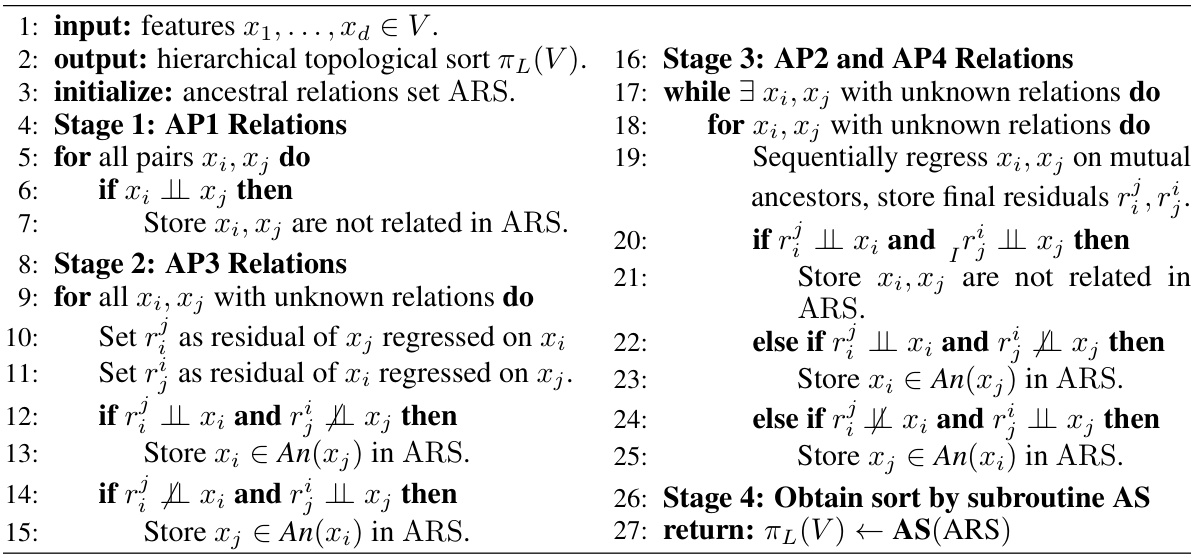
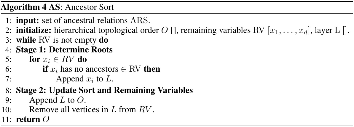
This algorithm details the steps for obtaining a linear hierarchical topological sort using local ancestral relationships. It starts by identifying pairs of vertices with specific ancestral relationships (AP1, AP2, AP3, and AP4) using conditional independence tests and sequential regressions. Then it uses a subroutine (AS) to construct the hierarchical sort based on the identified ancestral relationships.

In-depth insights
#

Hybrid Causal Discovery
#

The concept of “Hybrid Causal Discovery” represents a significant advancement in causal inference. It acknowledges the limitations of relying solely on either constraint-based methods (which excel at handling high-dimensional data but might struggle with complex functional relationships) or functional causal models (which offer unique identifiability under specific assumptions but might be computationally expensive or limited in scope). A hybrid approach strategically combines the strengths of both paradigms. For instance, a hybrid method might utilize a constraint-based approach to initially narrow down the search space of potential causal graphs, followed by a functional model to refine the graph based on specific functional form assumptions and evaluate the goodness-of-fit. This combination allows for efficient and accurate causal discovery in complex scenarios where neither method alone would suffice. The key is to carefully select the combination to leverage the best properties of each and mitigate their weaknesses. Careful attention must be given to the assumptions of each component and their interplay. This hybrid approach holds considerable promise for advancing causal discovery in various fields where data is high-dimensional and the underlying causal relationships might be non-linear and/or complex.

Topological Sorting
#

Topological sorting in causal discovery aims to order variables such that if variable A causes variable B, A precedes B in the ordering. This is crucial because it reduces the search space for causal relationships by eliminating impossible edge directions. The paper explores two novel topological sorting algorithms: one for linear models and another for nonlinear models. Both algorithms leverage local structural information, focusing on parent-child or ancestor-descendant relationships instead of relying on global properties. This is significant because it improves scalability and robustness by limiting the computational complexity associated with evaluating global relationships, especially in high-dimensional data. The linear algorithm uses ancestral relationships within the linear structural equation models to efficiently create a hierarchical ordering. This is computationally efficient while still capturing considerable causal information. The nonlinear algorithm, meanwhile, utilizes active causal paths to determine local parent-child relationships, demonstrating effectiveness even with arbitrary noise distributions. The nonparametric nature of these approaches enhances their robustness and applicability to a wider range of causal models. Overall, these methods present a valuable contribution to causal discovery by providing a more efficient and accurate approach to topological sorting.

Nonlinear ANM
#

Nonlinear Additive Noise Models (ANMs) present a significant challenge and opportunity in causal discovery. Linear ANMs, while offering theoretical elegance and computational tractability, often fail to capture the complexities of real-world systems where causal relationships are rarely linear. Nonlinear ANMs, therefore, become crucial for accurate causal inference in such scenarios. However, identifiability—ensuring a unique causal graph—becomes substantially more difficult with nonlinearities. This necessitates more sophisticated algorithms that can handle the increased complexity, often employing nonparametric methods or making stronger assumptions about the noise distribution. The paper’s approach to hybrid causal discovery, combining constraint-based methods with functional modeling, offers a potential pathway for addressing this challenge, particularly in high-dimensional settings. Exploiting local causal structures helps to overcome the curse of dimensionality often associated with nonlinear approaches. The success of this strategy hinges on identifying and leveraging conditions under which local relationships provide sufficient information for causal inference.

Edge Discovery Algo
#

An edge discovery algorithm, within the context of causal graphical models, aims to accurately identify the direct causal relationships between variables. Efficiency is crucial, as exhaustive searches are computationally expensive for large datasets. The algorithm likely leverages a topological ordering (a prioritized list of variables) to reduce the search space. This ordering informs the algorithm which variables to consider as potential parents of others, thus improving efficiency. The method may employ conditional independence testing to determine if a candidate edge truly represents a causal link, ruling out spurious correlations. Constraint-based approaches can further refine the output by pruning edges that violate pre-defined constraints. A well-designed edge discovery algorithm should be robust to noise and provide theoretical guarantees on its correctness and computational complexity. Non-parametric methods provide greater flexibility in handling nonlinear relationships but may require more data and computational resources than parametric methods. The choice of methods depends on the specific assumptions of the causal model, the characteristics of the data, and available computational resources.

Future Work
#

The paper’s “Future Work” section would ideally delve into several promising directions. Extending the algorithms to handle fully general additive noise models (ANMs), rather than restricting to the independent case or specific nonlinear forms, is crucial for broader applicability. This would involve addressing the complexities introduced by dependent noise terms and exploring robust estimation techniques. Another key area would be to improve the scalability of the algorithms for higher-dimensional datasets by investigating more efficient search strategies, such as incorporating parallel computing or approximate inference methods. Finally, it would be beneficial to explore applications to real-world data in diverse domains (e.g., genomics, climate science, social networks), validating the robustness and effectiveness of the proposed approach on complex datasets with potential confounding factors and missing data. Addressing these points would significantly strengthen the paper’s contribution to causal discovery.

More visual insights
#

More on figures

This figure illustrates the four possible relationships between two nodes (xi and xj) in terms of active causal paths. It shows different combinations of active frontdoor and backdoor paths. * AP1: No active path exists between xi and xj. * AP2: There is only an active backdoor path between xi and xj. * AP3: There is only an active frontdoor path between xi and xj. * AP4: There are both active frontdoor and backdoor paths between xi and xj. The dashed arrows represent ancestral relationships.

This figure shows the four possible types of active causal parental path relations between a variable and one of its parents, considering other parents of that variable. These relations are used in the nonlinear topological sorting algorithm (NHTS) to identify parent-child relationships.

This figure is a directed acyclic graph (DAG) used to illustrate Lemma 5.1 in the paper. The lemma provides a sufficient condition for determining whether a directed edge exists between two vertices, xi and xj, in a DAG. The DAG shows three vertices: xi, xj and a set of vertices denoted as Zij, where Zij = Cij U Mij. Cij represents potential confounders of xi and xj, and Mij represents potential mediators between xi and xj. The red arrow shows the direct edge between xi and xj that Lemma 5.1 is testing for. The lemma states that if xi and xj are conditionally independent given Zij, then there is no direct causal relationship between xi and xj. Conversely, if they are not conditionally independent given Zij, then there is a direct causal relationship (represented by the red arrow).

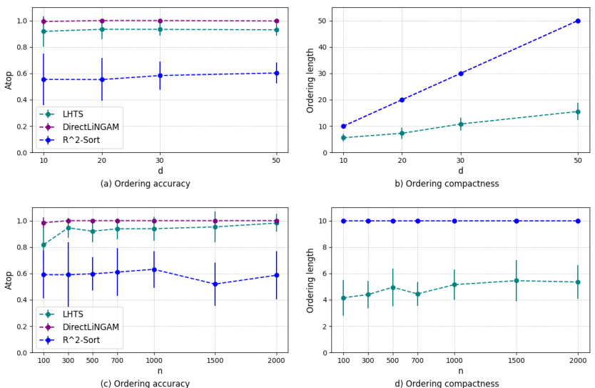
This figure shows the performance of the LHTS algorithm for linear topological sorting. The top row displays the ordering accuracy (Atop) and ordering compactness (ordering length) as a function of the dimension (d) of the data, with a fixed sample size (n=500). The bottom row shows the same metrics, but this time as a function of the sample size (n), holding the dimension fixed at d=10. The results are compared to two baseline algorithms, DirectLiNGAM and R^2-Sort. The appendix provides additional details on the runtime performance.

This figure shows the performance of the Nonlinear Hierarchical Topological Sort (NHTS) algorithm compared to other baseline methods (DirectLiNGAM, NoGAM, GES, GRaSP, GSP, and R2-Sort) on synthetic datasets. The datasets were generated with varying noise distributions (Gaussian, Laplace, and Uniform) and a fixed number of samples (n=300) and dimensions (d=10). The results demonstrate that NHTS outperforms the baseline methods in terms of ordering accuracy (Atop), a metric that represents the percentage of correctly ordered edges. Appendix D.2 provides additional runtime information for the experiments.

This figure shows the performance of the edge discovery algorithm (ED) on synthetic data with uniform noise. The left and middle panels display the F1-score of ED against dimension (d) with a fixed sample size (n=500), comparing it to Lasso, GAM, and RESIT. The right panel shows the F1-score against sample size (n) with a fixed dimension (d=10), also comparing it to Lasso and GAM (RESIT is excluded due to runtime issues at larger sample sizes). The results demonstrate that ED generally outperforms the baselines in terms of F1-score, especially as the dimension and sample size increase. Appendix D.5 provides further details on the runtime of the experiments.

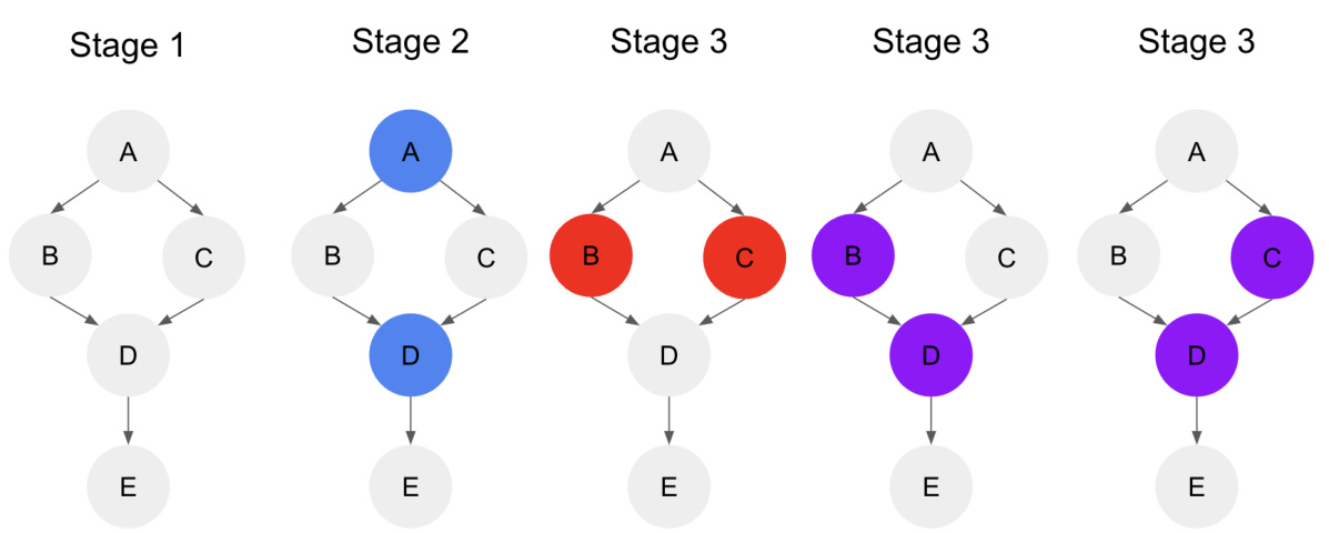
This figure shows the performance of the Linear Hierarchical Topological Sort (LHTS) algorithm on synthetic data. The top row illustrates the ordering accuracy (Atop) and compactness (ordering length) with a fixed sample size (n=500) and varying dimensions (d=10, 20, 30, 50). The bottom row displays the same metrics but with a fixed dimension (d=10) and varying sample sizes (n=100, 300, 500, 700, 1000, 1500, 2000). Appendix D.1 provides details on the runtime results.

This figure shows the performance of the LHTS algorithm for linear topological sorting. The top row displays the ordering accuracy (Atop) and ordering compactness (ordering length) for different dimensions (d) with a fixed sample size (n=500). The bottom row illustrates the same metrics but with a varying sample size (n) and a fixed dimension (d=10). Appendix D.1 provides additional details on the runtime performance.

This figure illustrates Lemma 5.1, which provides a sufficient condition for determining whether a directed edge exists between two nodes in a DAG given a topological ordering. It shows a DAG where the key is to show that the only active path from xi to xj is the direct edge, meaning there are no confounding or mediating effects. The conditioning set Zij ensures that only the direct causal effect from xi to xj is present, allowing for accurate determination of causality.

This figure shows the performance of the Nonlinear Hierarchical Topological Sort (NHTS) algorithm compared to other baseline methods (DirectLiNGAM, NoGAM, GES, GRaSP, GSP, and R2-Sort) across different noise distributions (Gaussian, Laplace, and Uniform). The results demonstrate NHTS’s superior performance in terms of topological ordering accuracy (Atop) for various scenarios. Appendix D.2 provides the runtimes for these experiments.

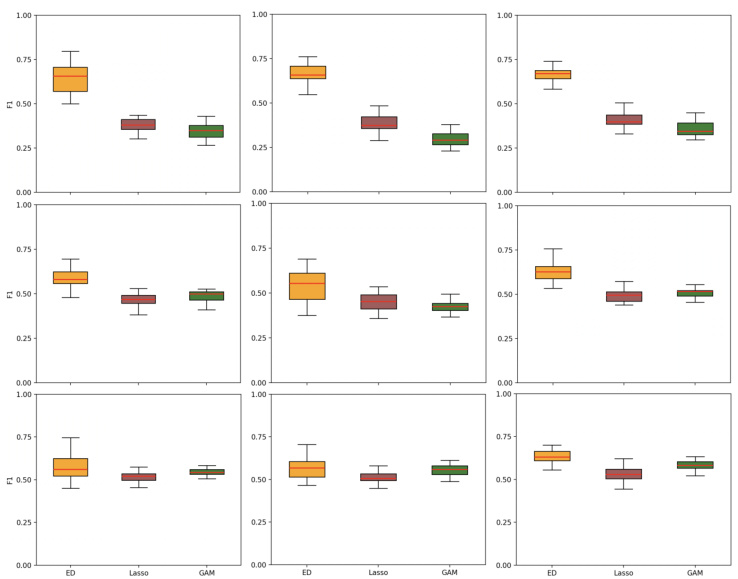
This figure shows the performance of the ED (Edge Discovery) algorithm on synthetic data with different noise distributions (Gaussian, Laplace, Uniform) and varying graph densities (average number of edges 2d, 3d, 4d). The box plots illustrate the F1-score achieved by ED, compared against Lasso and GAM (Generalized Additive Models) baselines. The results demonstrate ED’s performance across different noise types and graph densities, highlighting its robustness and effectiveness in causal discovery.