↗ OpenReview ↗ NeurIPS Homepage ↗ Chat
TL;DR#
Current neural network (NN)-based soft sensors prioritize offline accuracy over online stability and interpretability. This limitation hinders real-time applications where reliable and stable performance is critical. Existing training techniques, such as early stopping and adaptive learning rates, are unsuitable for online deployment, often leading to considerable performance drops. The paper addresses this gap by introducing a new framework.
The paper introduces the Approximated Orthogonal Projection Unit (AOPU), a novel NN architecture designed for stable training. AOPU minimizes variance estimation (MVE) by truncating the gradient backpropagation at dual parameters, optimizing updates, and enhancing robustness. AOPU also approximates natural gradient descent (NGD), a computationally expensive method, making it feasible for NN optimization. Empirical results demonstrate superior stability and performance compared to existing methods. The Rank Ratio metric quantifies the heterogeneity of training data and is used to better understand model performance.
Key Takeaways#
Why does it matter?#
This paper is crucial for researchers in industrial soft sensor applications and deep learning optimization. It addresses the critical need for stable online training of neural networks, a major challenge in industrial settings. The proposed AOPU method offers a novel solution with a strong theoretical foundation, paving the way for improved safety, reliability, and efficiency of industrial processes. Its innovative approach to approximating natural gradient descent, combined with interpretability measures, opens exciting new avenues for future research in this field.
Visual Insights#

This figure compares two neural network structures: a conventional deep neural network (DNN) and a broad learning system (BLS). The key difference highlighted is the distinction between ’trackable’ and ‘untrackable’ parameters. Trackable parameters are those directly involved in the linear transformation of inputs to outputs, represented by solid green lines. Untrackable parameters, shown by orange curves, represent non-linear operations like activation functions that are not directly part of the linear transformation process. The figure illustrates how the BLS structure modifies the DNN by introducing an augmentation block that generates additional features, leading to a more robust feature extraction and potentially better approximation of the Minimum Variance Estimator (MVE).
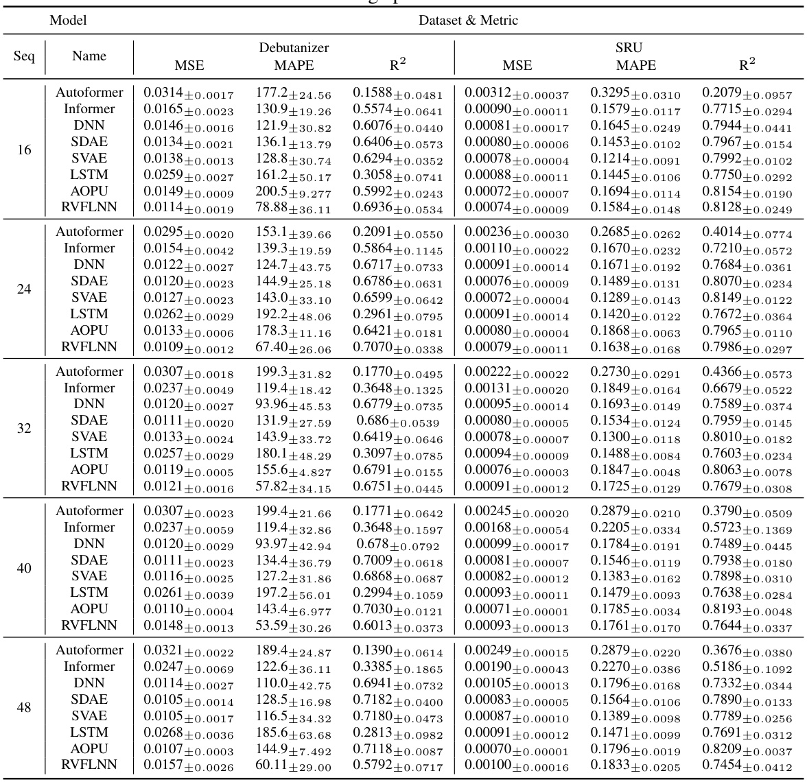
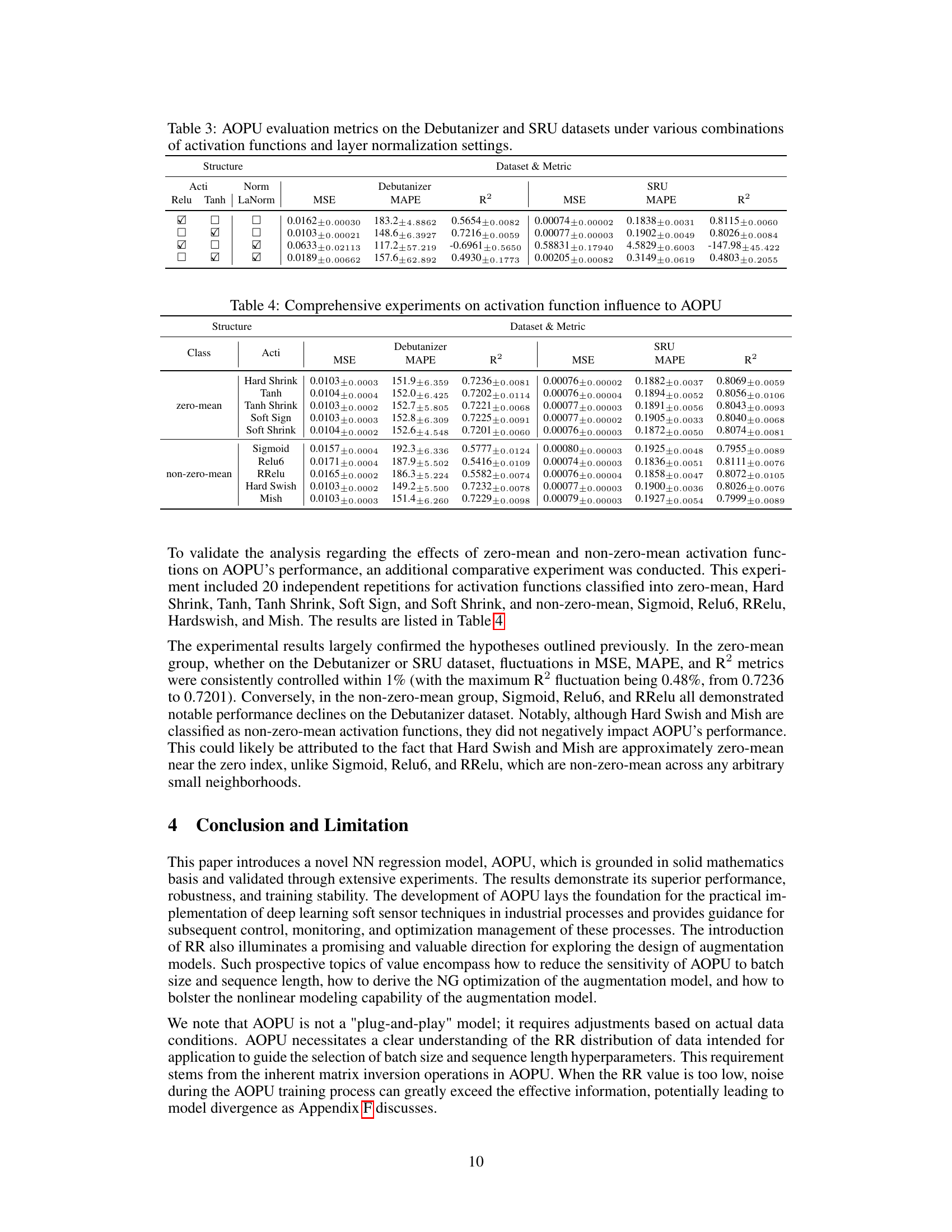
This table presents the performance of different models (Autoformer, Informer, DNN, SDAE, SVAE, LSTM, AOPU, and RVFLNN) on two datasets (Debutanizer and SRU) for various sequence lengths. The models are evaluated using MSE, MAPE, and R². The best training epoch is selected for each model and sequence length. The batch size (bs) is fixed at 64.
In-depth insights#
AOPU: MVE Approx#
The heading ‘AOPU: MVE Approx’ suggests a discussion of how the Approximated Orthogonal Projection Unit (AOPU) approximates Minimum Variance Estimation (MVE). This likely involves explaining the mathematical underpinnings of AOPU, demonstrating how it leverages properties of orthogonal projections and truncated gradients to achieve an efficient, stable approximation of MVE, especially in scenarios involving high-dimensional data or complex models where exact MVE calculation is computationally prohibitive. A key aspect would be to show how the approximation impacts the training stability and the model’s overall performance, perhaps by comparing it to standard gradient descent methods and other related techniques. The analysis would likely highlight the tradeoffs between computational efficiency and accuracy of the MVE approximation, possibly providing empirical evidence that the approximation is sufficiently accurate for practical applications, especially in the context of industrial soft sensors where stable online operation is paramount. Finally, the discussion might delve into the interpretation of the AOPU’s output as an approximation of the MVE estimator, linking it to broader statistical concepts and its implications for model interpretability and reliability.
Stable NN Training#
Stable training of neural networks (NNs) is crucial for reliable performance, especially in applications demanding real-time predictions and robustness to noisy data or fluctuating conditions. This paper delves into techniques for achieving stable NN training, focusing on the impact of minimizing variance in parameter estimation. Approximated Orthogonal Projection Units (AOPUs) are introduced as a novel NN architecture designed to stabilize the training process. AOPUs cleverly truncate the gradient backpropagation, which helps achieve stability. The core idea centers around approximating the minimum variance estimator (MVE) within the NN framework. The concept of trackable versus untrackable parameters within the NN is introduced, forming the theoretical foundation of the proposed method. By strategically focusing on the optimization of trackable parameters, AOPUs mitigate the impact of untrackable parameters’ variability on the training process, making it more stable. Rank Ratio (RR), an interpretability index, is also introduced to quantify the linear independence of samples and predict training performance. The experimental results demonstrate significant performance improvements for AOPUs compared to other state-of-the-art NNs in achieving stable convergence. The key is to balance model capacity with the need for robust training; over-parameterization can increase instability despite higher accuracy.
Dual Parameter Update#
The concept of “Dual Parameter Update” in the context of the provided research paper, likely refers to a training methodology that employs two sets of parameters: trackable and untrackable. The trackable parameters are directly optimized during the training process, while the untrackable parameters, influenced by activation functions, are indirectly updated. This dual approach likely aims to approximate the Natural Gradient Descent (NGD) method while mitigating its computational cost. By truncating backpropagation at the dual parameters and optimizing the trackable parameters based on truncated gradients, the model effectively approximates Minimum Variance Estimation (MVE). The dual parameter update method enhances training stability and robustness by focusing on stable convergence rather than solely prioritizing accuracy. The use of a rank ratio (RR) metric further provides an interpretability index to gauge the quality of the approximation and to predict training performance. The effectiveness hinges on the assumption that the features are well-extracted, making it essential to utilize robust feature extraction methods and data augmentation techniques.
Rank Ratio (RR)#
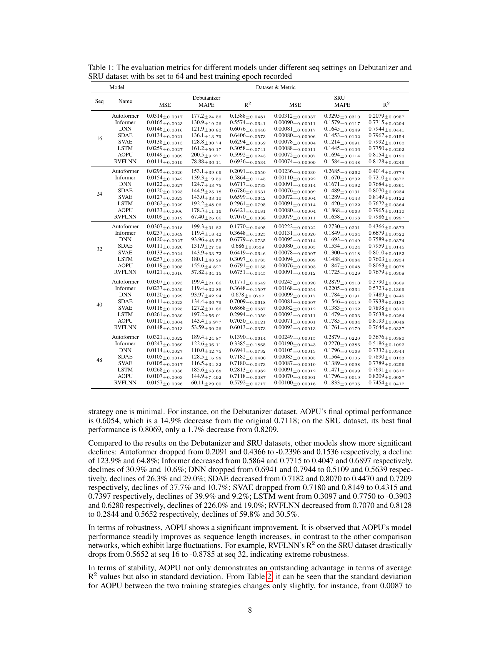
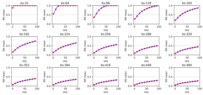
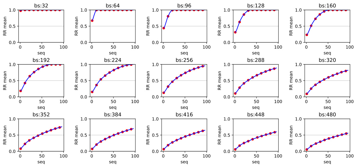
The Rank Ratio (RR) serves as a crucial interpretability index within the Approximated Orthogonal Projection Unit (AOPU) framework. It quantifies the ratio of linearly independent samples within each mini-batch, effectively measuring the data heterogeneity and diversity. A high RR (close to 1) indicates that the model’s output closely approximates the Minimum Variance Estimation (MVE), aligning optimization more closely with the Natural Gradient Descent (NGD). This suggests superior performance and stability. Conversely, a low RR (close to 0) implies compromised computational precision and suboptimal performance. RR’s value dynamically influences AOPU’s convergence, with high RR values leading to stable convergence and low RR values resulting in unstable or non-convergent behavior. Therefore, monitoring RR during training provides valuable insights into the model’s dynamics and can help predict performance and identify potential issues early on. RR acts as a critical indicator of AOPU’s approximation fidelity to MVE and NGD, which are key theoretical underpinnings of AOPU’s superior performance.
AOPU Limitations#
The Approximated Orthogonal Projection Unit (AOPU) model, while demonstrating strong performance and stability in regression tasks, is not without limitations. A core limitation is its dependence on the Rank Ratio (RR) to ensure numerical stability and convergence. A low RR, which can occur with larger batch sizes or shorter sequence lengths, can lead to computational issues and model instability. This highlights a trade-off between batch size, sequence length, and AOPU’s effective approximation of the Natural Gradient. Furthermore, the model’s performance is sensitive to the choice of the data augmentation module and activation functions, underscoring the need for careful hyperparameter tuning. While AOPU exhibits superior stability compared to other methods, it is not a purely plug-and-play model and requires careful consideration of data characteristics and hyperparameter settings for optimal deployment. Finally, AOPU’s theoretical foundation relies on assumptions that may not always hold in real-world data, particularly concerning the linear independence of data samples and normality of noise.
More visual insights#
More on figures

The figure shows the data flow of the Approximated Orthogonal Projection Unit (AOPU) model. Input data is first processed, likely through a feature extraction module (not explicitly shown). The core of the AOPU involves ’trackable’ and ‘dual’ parameters. The gradient is calculated based on the objective function and backpropagated, but this propagation stops at the dual parameter. The gradient information at the dual parameter is then used to update the trackable parameters. This process is shown to approximate the natural gradient. The updated trackable parameters then lead to a final prediction which is compared to the actual output data, influencing the next iteration.
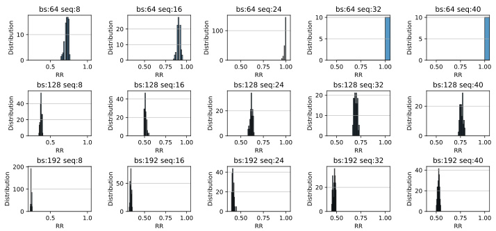
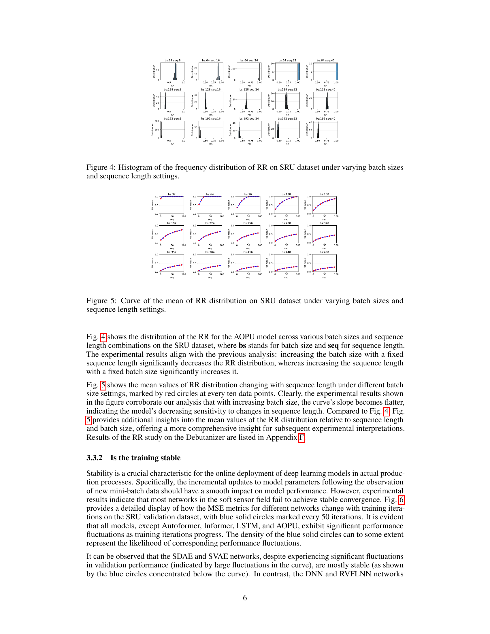
This figure shows the distribution of the Rank Ratio (RR) for different batch sizes and sequence lengths on the SRU dataset. Each subplot is a histogram representing the frequency distribution of RR for a specific combination of batch size and sequence length. The x-axis represents the RR values, and the y-axis represents the frequency. The figure helps to visualize how the RR changes with varying batch sizes and sequence lengths. Analyzing this data provides insight into the robustness and stability of the AOPU model under different data characteristics.
This figure displays histograms showing the distribution of the Rank Ratio (RR) for various batch sizes and sequence lengths on the SRU dataset. The histograms reveal how the RR values are distributed across different experimental conditions. By observing the shape and spread of the histograms, one can gain insights into the impact of batch size and sequence length on the stability and performance of the AOPU model, as described in the paper.
This figure shows the schematic diagrams of two industrial processes: the Sulfur Recovery Unit (SRU) and the Debutanizer. The SRU diagram (a) illustrates the flow of gas (MEA gas and SWS gas) and air through various chambers for combustion and sulfur recovery. The Debutanizer diagram (b) depicts the process flow of a desulfurizing and naphtha splitter plant. It focuses on the flow and temperature within the Debutanizer column, highlighting the points where sensor measurements are taken (as described in Table 5). Both diagrams visually represent the processes and the location of the sensor measurements which are used as input data for the soft sensor models developed and discussed in the paper.

This figure compares two neural network architectures: a conventional deep neural network and a broad learning system. The key difference highlighted is the distinction between ’trackable’ and ‘untrackable’ parameters. Trackable parameters are directly linked to the model’s weights and can be updated during training, while untrackable parameters are implicitly defined by non-parametric operations (shown as orange curves) and their values cannot be directly tracked or optimized. The broad learning system (b) incorporates data enhancement, suggesting a potential method for improving model performance or stability. The figure illustrates how AOPU (Approximated Orthogonal Projection Unit) approaches the problem of parameter optimization using a hybrid of conventional and broad learning elements.

This figure shows the schematic diagrams of two industrial processes, SRU (Sulfur Recovery Unit) and Debutanizer, which are used as datasets in the paper’s experiments. The diagrams illustrate the flow of materials and the locations of sensors used to collect data for the soft sensor models discussed in the paper. The SRU diagram (a) shows the process of removing pollutants from acid gas streams before they are released into the atmosphere, involving multiple chambers and air flows, while the Debutanizer diagram (b) details the process of maximizing C5 (stabilized gasoline) and minimizing C4 (butane) content in a desulfuring and naphtha splitter plant.
This figure shows the schematic diagrams of two industrial processes: the Sulfur Recovery Unit (SRU) and the Debutanizer. The SRU diagram (a) illustrates the flow of gases (MEA gas, air, and SWS gas) through various chambers and processes involved in sulfur recovery. The Debutanizer diagram (b) depicts a column used in desulfurization and naphtha splitting, showing the flow of materials and temperature points.

This figure shows the schematic diagrams of two industrial processes: the Sulfur Recovery Unit (SRU) and the Debutanizer. The SRU diagram (a) illustrates the flow of gases (MEA GAS, AIR_MEA, AIR_MEA_2, SWS) through various units and chambers. The Debutanizer diagram (b) displays the flow of materials within a column, including the top and bottom temperatures and flows. These diagrams help to visualize the physical context in which the AOPU model is applied and the data used in model training originates.
This figure shows the schematic diagrams of two industrial processes: the Sulfur Recovery Unit (SRU) and the Debutanizer. The SRU diagram (a) illustrates the flow of gas (MEA_GAS and SWS), air (AIR_MEA and AIR_SWS), and the resulting sulfur product. The Debutanizer diagram (b) shows the process flow, including inputs, temperatures, and outputs from a Debutanizer column used in petroleum refining. These diagrams provide a visual representation of the complex processes and the locations of the sensors used in data collection for the study described in the paper.
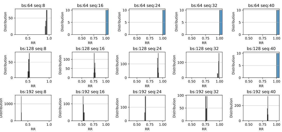
This figure displays histograms showing the distribution of the Rank Ratio (RR) metric for different batch sizes and sequence lengths on the SRU dataset. Each histogram represents a specific combination of batch size and sequence length. The x-axis shows the RR values, and the y-axis shows the frequency of those values in the dataset for that specific setting. The figure is intended to illustrate the effect of batch size and sequence length on the RR metric.
This figure displays histograms showing the distribution of the Rank Ratio (RR) metric for the SRU dataset. The histograms are generated by varying both the batch size and the sequence length. Each subplot represents a different combination of batch size and sequence length. This helps visualize how different input data characteristics affect the RR values and the stability of the AOPU model during training.
This figure shows the schematic diagrams of two industrial processes: a sulfur recovery unit (SRU) and a debutanizer. The SRU diagram (a) illustrates the flow of MEA gas, air, and secondary air, and the debutanizer diagram (b) shows the temperature and pressure measurements at different points of the process.
This figure compares the structures of conventional deep neural networks and broad learning systems. It highlights the distinction between ’trackable’ parameters (which can be directly calculated from input data) and ‘untrackable’ parameters (influenced by activation functions, etc.). The figure shows how the broad learning system incorporates data augmentation to create an enhanced input for the model. This is relevant to the paper’s proposed method AOPU, which aims to improve training stability by leveraging trackable parameters.

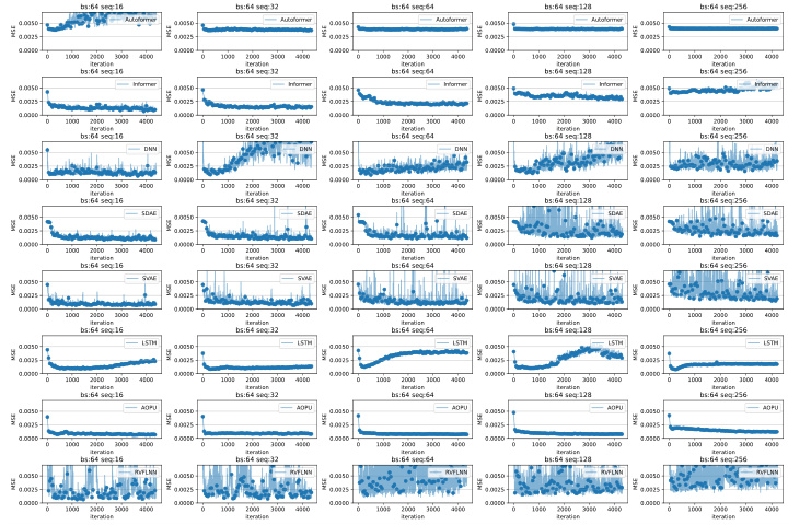
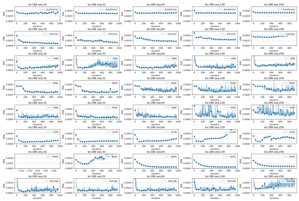
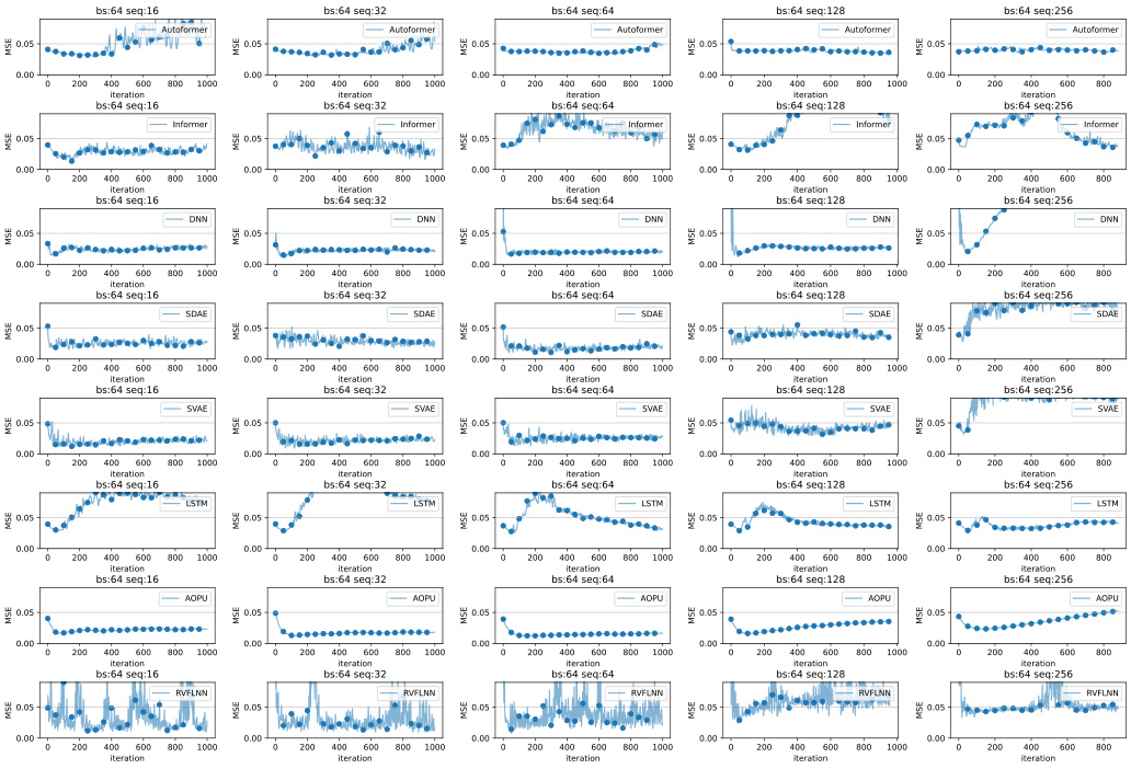
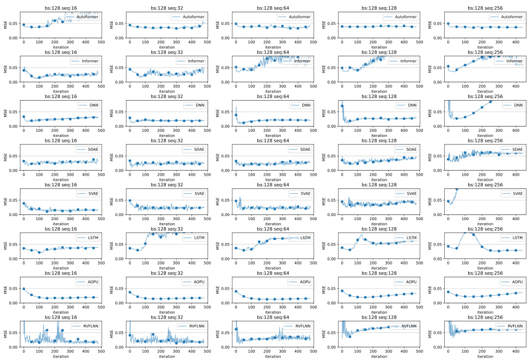
This figure displays the validation loss curves of several models (Autoformer, Informer, DNN, SDAE, SVAE, LSTM, AOPU, and RVFLNN) trained on the SRU dataset. The plots show how the validation loss changes over training iterations for different sequence lengths (16, 32, 64, 128, 256) while keeping the batch size constant at 128. This visualization helps in assessing the stability and convergence speed of each model under varying sequence lengths. The goal is to evaluate which model exhibits the most stable and rapid convergence to a low validation loss.
More on tables
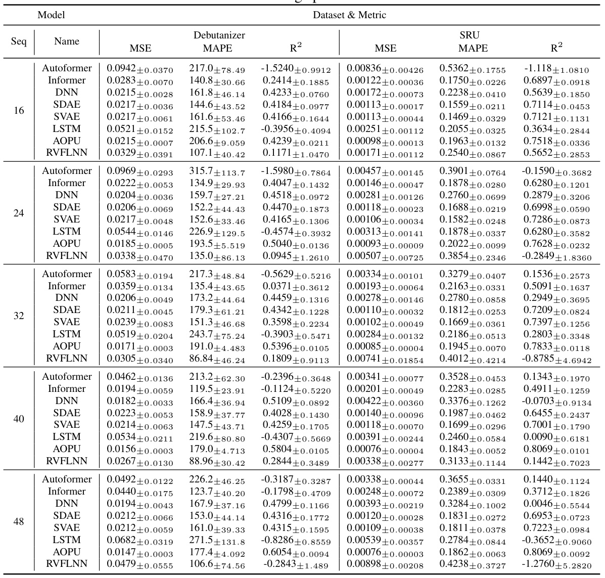
This table presents the performance evaluation of different models (Autoformer, Informer, DNN, SDAE, SVAE, LSTM, AOPU, and RVFLNN) on two datasets (Debutanizer and SRU) using various sequence lengths. The evaluation metrics include MSE (Mean Squared Error), MAPE (Mean Absolute Percentage Error), and R². The best-performing epoch for each model and sequence length combination is selected. This allows for a direct comparison of models based on their optimal performance. The results show a comparison of different models’ performance at their best epoch with a batch size of 64 and the effect of sequence length.

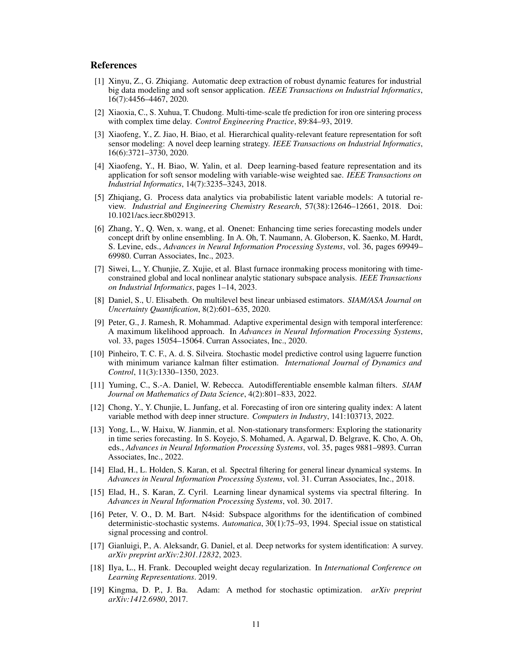
This table presents the results of an ablation study on the AOPU model. It shows the Mean Squared Error (MSE), Mean Absolute Percentage Error (MAPE), and R-squared (R²) values achieved by AOPU on the Debutanizer and SRU datasets, under different combinations of activation functions (Relu, Tanh) and layer normalization (LaNorm). Each row represents a different configuration of activation functions and layer normalization, allowing the reader to assess the impact of these design choices on the model’s performance.

This table presents the performance evaluation of different models (Autoformer, Informer, DNN, SDAE, SVAE, LSTM, AOPU, and RVFLNN) on two datasets (Debutanizer and SRU) using different sequence lengths. The batch size is fixed at 64. The best training epoch for each model configuration is selected and used to report metrics such as MSE, MAPE, and R². The table helps to compare the performance of AOPU against established baselines.

This table presents the performance comparison of different models (Autoformer, Informer, DNN, SDAE, SVAE, LSTM, AOPU, and RVFLNN) on two datasets (Debutanizer and SRU). The models were trained using Mean Squared Error (MSE) loss, except AOPU which uses approximated minimum variance estimation. The table shows MSE, MAPE, and R-squared values for each model and sequence length. The best performing epoch was selected for this comparison. The batch size was fixed at 64 for all models. The results provide a quantitative analysis of AOPU’s performance against established baselines.

This table presents the performance evaluation metrics for various soft sensor models on two different datasets (Debutanizer and SRU). The metrics used are Mean Squared Error (MSE), Mean Absolute Percentage Error (MAPE), and R-squared (R2). Different sequence lengths (‘seq’) are considered while keeping the batch size (‘bs’) constant at 64. The table shows the results for each model at its best performing epoch during training.

This table presents a comparison of different models’ performance on two datasets (Debutanizer and SRU) using various sequence lengths. The models are evaluated using MSE (Mean Squared Error), MAPE (Mean Absolute Percentage Error), and R². The best training epoch for each model and sequence length combination is used for the evaluation. The table shows the mean and standard deviation of the metrics across multiple runs.
Full paper#
